pymaid
Overview
pymaid lets you interface with a CATMAID server. It’s built on top of navis and returns data (neurons, volumes) in a way that you can plug them straight into navis to use features such as plotting.
Official documentation here.
Connecting
The VFB CATMAID servers (see here for what’s available) are public and don’t require an API token for read-only access which makes connecting simple:
import pymaid
import navis
navis.set_pbars(jupyter=False)
pymaid.set_pbars(jupyter=False)
# Connect to the VFB CATMAID server hosting the FAFB data
rm = pymaid.connect_catmaid(server="https://fafb.catmaid.virtualflybrain.org/", api_token=None, max_threads=10)
# Test call to see if connection works
print(f'Server is running CATMAID version {rm.catmaid_version}')
WARNING: Could not load OpenGL library.
INFO : Global CATMAID instance set. Caching is ON. (pymaid)
Server is running CATMAID version 2020.02.15-905-g93a969b37
Retrieving neurons
Let’s start with pulling a neuron based on its ID:
# Find a neuron from its ID (16) -> this is an olfactory projection neuron
n = pymaid.get_neurons(16)
n
| type | CatmaidNeuron |
|---|---|
| name | Uniglomerular mALT VA6 adPN 017 DB |
| id | 16 |
| n_nodes | 16840 |
| n_connectors | 2158 |
| n_branches | 1172 |
| n_leafs | 1230 |
| cable_length | 4003103.232861 |
| soma | [2941309] |
| units | 1 nanometer |
This neuron’s type is pymaid.CatmaidNeuron, which is a subclass of navis.TreeNeuron. The list version is pymaid.CatmaidNeuronList, which a subclass of navis.NeuronList. This adds a bit of extra functionality (such as lazy loading of data) and allows CatmaidNeuron and CatmaidNeuronList work as drop in replacements for their parent classes.
# Plot CatmaidNeuron with navis
navis.plot3d(n, width=1000, connectors=True, c='k')
get_neurons() returns neurons including their “connectors” - i.e. pre- (red) and postsynapses (blue). For this particular neuron, the published data comprehensively labels the axonal synapses but not the dendrites. Analogous to the nodes table, you can access the connectors like so:
n.connectors.head()
| node_id | connector_id | type | x | y | z | |
|---|---|---|---|---|---|---|
| 0 | 97891 | 97895 | 0 | 436882.09375 | 161840.453125 | 212160.0 |
| 1 | 2591 | 97954 | 0 | 437120.00000 | 160998.000000 | 211920.0 |
| 2 | 2665 | 98300 | 0 | 437183.75000 | 162323.515625 | 214880.0 |
| 3 | 2646 | 98373 | 0 | 437041.68750 | 162451.937500 | 214120.0 |
| 4 | 2654 | 98415 | 0 | 436760.90625 | 163689.796875 | 214440.0 |
Let’s run a bigger example and pull all data published with Bates, Schlegel et al. 2020. For this, we will use “annotations”. These are effectively text labels that group neurons together, in this case by paper. Instead of get_neurons we can use find_neurons to avoid downloading unnecessary data.
bates = pymaid.find_neurons(annotations='Paper: Bates and Schlegel et al 2020')
len(bates)
INFO : Found 583 neurons matching the search parameters (pymaid)
583
bates is a CatmaidNeuronList containing 583 neurons. Importantly pymaid has not yet loaded any data other than names! Note all the “NAs” in the summary:
bates.head()
| type | name | skeleton_id | n_nodes | n_connectors | n_branches | n_leafs | cable_length | soma | units | |
|---|---|---|---|---|---|---|---|---|---|---|
| 0 | CatmaidNeuron | Uniglomerular mALT DA1 lPN 57316 2863105 ML | 2863104 | NA | NA | NA | NA | NA | NA | 1 nanometer |
| 1 | CatmaidNeuron | Uniglomerular mALT DA3 adPN 57350 HG | 57349 | NA | NA | NA | NA | NA | NA | 1 nanometer |
| 2 | CatmaidNeuron | Uniglomerular mALT DA1 lPN 57354 GA | 57353 | NA | NA | NA | NA | NA | NA | 1 nanometer |
| 3 | CatmaidNeuron | Uniglomerular mALT VA6 adPN 017 DB | 16 | NA | NA | NA | NA | NA | NA | 1 nanometer |
| 4 | CatmaidNeuron | Uniglomerular mALT VA5 lPN 57362 ML | 57361 | NA | NA | NA | NA | NA | NA | 1 nanometer |
We could have used pymaid.get_neurons(annotations='Paper: Bates and Schlegel et al 2020') instead to load all data up-front, but this would increase memory usage.
The CatmaidNeuronList we have created will lazy load data from the server when required.
# Access the first neuron's nodes
# -> this will trigger a data download
_ = bates[0].nodes
# Run summary again
bates.head()
| type | name | skeleton_id | n_nodes | n_connectors | n_branches | n_leafs | cable_length | soma | units | |
|---|---|---|---|---|---|---|---|---|---|---|
| 0 | CatmaidNeuron | Uniglomerular mALT DA1 lPN 57316 2863105 ML | 2863104 | 6774 | 470 | 280 | 292 | 1522064.513255 | [3245741] | 1 nanometer |
| 1 | CatmaidNeuron | Uniglomerular mALT DA3 adPN 57350 HG | 57349 | NA | NA | NA | NA | NA | NA | 1 nanometer |
| 2 | CatmaidNeuron | Uniglomerular mALT DA1 lPN 57354 GA | 57353 | NA | NA | NA | NA | NA | NA | 1 nanometer |
| 3 | CatmaidNeuron | Uniglomerular mALT VA6 adPN 017 DB | 16 | NA | NA | NA | NA | NA | NA | 1 nanometer |
| 4 | CatmaidNeuron | Uniglomerular mALT VA5 lPN 57362 ML | 57361 | NA | NA | NA | NA | NA | NA | 1 nanometer |
We have now loaded data for the first neuron.
Next we willl find and plot all uniglomelar DA1 projection neurons by their name.
# Name will be match pattern "Uniglomerular {tract} DA1 {lineage}"
import re
prog = re.compile("Uniglomerular(.*?) DA1 ")
# Match all neuron names in `bates` against that pattern
is_da1 = list(map(lambda x: prog.match(x) != None, bates.name))
# Subset list
da1 = bates[is_da1]
da1.head()
| type | name | skeleton_id | n_nodes | n_connectors | n_branches | n_leafs | cable_length | soma | units | |
|---|---|---|---|---|---|---|---|---|---|---|
| 0 | CatmaidNeuron | Uniglomerular mALT DA1 lPN 57316 2863105 ML | 2863104 | 6774 | 470 | 280 | 292 | 1522064.513255 | [3245741] | 1 nanometer |
| 1 | CatmaidNeuron | Uniglomerular mALT DA1 lPN 57354 GA | 57353 | NA | NA | NA | NA | NA | NA | 1 nanometer |
| 2 | CatmaidNeuron | Uniglomerular mALT DA1 lPN 57382 ML | 57381 | NA | NA | NA | NA | NA | NA | 1 nanometer |
| 3 | CatmaidNeuron | Uniglomerular mlALT DA1 vPN mlALTed Milk 23348... | 2334841 | NA | NA | NA | NA | NA | NA | 1 nanometer |
| 4 | CatmaidNeuron | Uniglomerular mALT DA1 lPN PN021 2345090 DB RJVR | 2345089 | NA | NA | NA | NA | NA | NA | 1 nanometer |
# Plot neurons by their lineage
for n in da1:
# Split name into components and keep the lineage
n.lineage = n.name.split(' ')[3]
# Generate a color per lineage
import seaborn as sns
import numpy as np
lineages = np.unique(da1.lineage)
lin_cmap = dict(zip(lineages, sns.color_palette('muted', len(lineages))))
neuron_cmap = {n.id: lin_cmap[n.lineage] for n in da1}
navis.plot3d(da1, color=neuron_cmap, hover_name=True)
Let’s add the neuropil meshes. These are called “volumes” on the CATMAID servers. To find out what’s available:
vols = pymaid.get_volume()
vols.head()
INFO : Retrieving list of available volumes. (pymaid)
| id | name | comment | user_id | editor_id | project_id | creation_time | edition_time | annotations | area | volume | watertight | meta_computed | |
|---|---|---|---|---|---|---|---|---|---|---|---|---|---|
| 0 | 439 | v14.neuropil | None | 55 | 247 | 1 | 2017-10-05T21:01:18.683Z | 2018-08-30T17:21:20.910Z | None | 6.377313e+11 | 1.533375e+16 | False | True |
| 1 | 440 | AME_R | Accessory medulla right | 55 | 55 | 1 | 2017-10-08T13:54:03.279Z | 2017-10-08T13:54:03.279Z | None | 1.894095e+09 | 4.799292e+12 | True | True |
| 2 | 441 | LO_R | Lobula right | 55 | 55 | 1 | 2017-10-08T13:54:03.840Z | 2017-10-08T13:54:03.840Z | None | 4.103282e+10 | 5.790708e+14 | True | True |
| 3 | 442 | NO | Noduli | 55 | 55 | 1 | 2017-10-08T13:54:04.084Z | 2017-10-08T13:54:04.084Z | None | 3.955158e+09 | 1.796395e+13 | True | True |
| 4 | 443 | BU_R | Bulb right | 55 | 55 | 1 | 2017-10-08T13:54:04.263Z | 2017-10-08T13:54:04.263Z | None | 1.445868e+09 | 4.109262e+12 | True | True |
# Get the neuropil volume
v14neuropil = pymaid.get_volume('v14.neuropil')
# Make it slightly more transparent
v14neuropil.color = (.8, .8, .8, .3)
INFO : Cached data used. Use `pymaid.clear_cache()` to clear. (pymaid)
# Plot with neuropil volume
navis.plot3d([da1, v14neuropil], color=neuron_cmap)
Suggested exercises:
- find all uniglomerular projection neurons (name starts with
Uniglomerular) - calculate the number of pre-/post-synapses in the right lateral horn (LH) (use
pymaid.get_volumeandnavis.in_volume) - group the neurons by glomerulus based on label (nomenclature is
Uniglomerular {tract} {glomerulus} {lineage} {metadata}) - plot LH pre- vs post-synapses in a scatter plot (e.g. using
seaborn.scatterplot)
Pulling connectivity
CATMAID lets you fetch connectivity data either as a list of up- and downstream partners or as whole adjacency matrices.
# Pull downstream partners of DA1 PNs
da1_ds = pymaid.get_partners(da1,
threshold=3, # anything with >= 3 synapses
directions=['outgoing'] # downstream partners only
)
# Result is a pandas DataFrame
da1_ds.head()
INFO : Fetching connectivity table for 17 neurons (pymaid)
INFO : Done. Found 0 pre-, 270 postsynaptic and 0 gap junction-connected neurons (pymaid)
| neuron_name | skeleton_id | num_nodes | relation | 2863104 | 57353 | 57381 | 2334841 | 2345089 | 27295 | ... | 2319457 | 4207871 | 755022 | 2379517 | 61221 | 3239781 | 2381753 | 57311 | 57323 | total | |
|---|---|---|---|---|---|---|---|---|---|---|---|---|---|---|---|---|---|---|---|---|---|
| 0 | Uniglomerular mlALT DA1 vPN mlALTed Milk 18114... | 1811442 | 11769 | downstream | 30 | 3 | 4 | 0 | 0 | 15 | ... | 0 | 0 | 32 | 0 | 26 | 0 | 0 | 21 | 20 | 151.0 |
| 1 | Uniglomerular mlALT DA1 vPN mlALTed Milk 23348... | 2334841 | 6362 | downstream | 0 | 0 | 0 | 0 | 14 | 0 | ... | 22 | 17 | 0 | 28 | 0 | 26 | 32 | 0 | 0 | 139.0 |
| 2 | LHAV4a4#1 1911125 FML PS RJVR | 1911124 | 6969 | downstream | 23 | 6 | 9 | 0 | 0 | 5 | ... | 0 | 0 | 19 | 0 | 13 | 0 | 0 | 19 | 15 | 109.0 |
| 3 | LHAV2a3#1 1870231 RJVR AJES PS | 1870230 | 14820 | downstream | 5 | 23 | 28 | 0 | 0 | 10 | ... | 0 | 0 | 19 | 0 | 7 | 0 | 0 | 5 | 7 | 105.0 |
| 4 | LHAV4c1#1 488056 downstream DA1 GSXEJ | 488055 | 12137 | downstream | 15 | 3 | 0 | 0 | 0 | 16 | ... | 0 | 0 | 15 | 0 | 15 | 0 | 0 | 17 | 11 | 92.0 |
5 rows × 22 columns
Each row is a synaptic downstream partner of our query DA1 neurons. The columns to the left contain the synapses they receive from individual query neurons. For example 1811442 (first row) receives 30 synapses from the DA1 PN with ID 2863104.
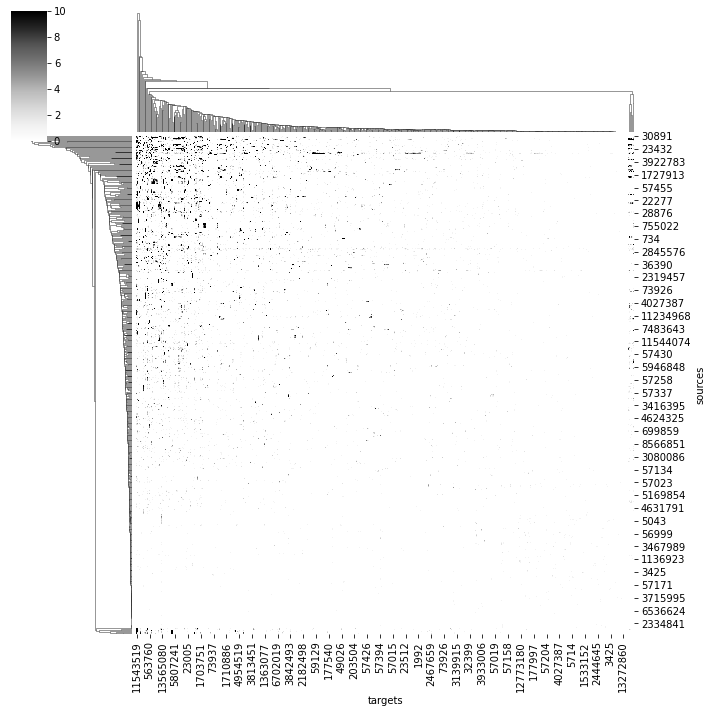
# Get an adjacency matrix between all Bates, Schlegel et al. neurons
adj = pymaid.adjacency_matrix(bates)
adj.head()
| targets | 2863104 | 57349 | 57353 | 16 | 57361 | 15738898 | 57365 | 4182038 | 3813399 | 11524119 | ... | 57323 | 4624362 | 1853423 | 2842610 | 57333 | 4624374 | 3080183 | 57337 | 4624378 | 57341 |
|---|---|---|---|---|---|---|---|---|---|---|---|---|---|---|---|---|---|---|---|---|---|
| sources | |||||||||||||||||||||
| 2863104 | 0.0 | 0.0 | 0.0 | 0.0 | 0.0 | 0.0 | 0.0 | 0.0 | 0.0 | 0.0 | ... | 2.0 | 0.0 | 12.0 | 0.0 | 0.0 | 0.0 | 0.0 | 0.0 | 0.0 | 0.0 |
| 57349 | 0.0 | 0.0 | 0.0 | 0.0 | 0.0 | 0.0 | 0.0 | 0.0 | 0.0 | 0.0 | ... | 0.0 | 0.0 | 0.0 | 0.0 | 0.0 | 0.0 | 0.0 | 0.0 | 0.0 | 0.0 |
| 57353 | 0.0 | 0.0 | 0.0 | 0.0 | 0.0 | 0.0 | 0.0 | 0.0 | 0.0 | 0.0 | ... | 0.0 | 0.0 | 5.0 | 0.0 | 0.0 | 0.0 | 0.0 | 0.0 | 0.0 | 0.0 |
| 16 | 0.0 | 0.0 | 0.0 | 1.0 | 0.0 | 0.0 | 0.0 | 0.0 | 0.0 | 1.0 | ... | 0.0 | 0.0 | 0.0 | 0.0 | 0.0 | 0.0 | 0.0 | 0.0 | 0.0 | 0.0 |
| 57361 | 0.0 | 0.0 | 0.0 | 0.0 | 0.0 | 0.0 | 0.0 | 0.0 | 0.0 | 0.0 | ... | 0.0 | 0.0 | 0.0 | 0.0 | 0.0 | 0.0 | 0.0 | 0.0 | 0.0 | 0.0 |
5 rows × 583 columns
# Plot a quick & dirty adjacency matrix
import seaborn as sns
ax = sns.clustermap(adj, vmax=10, cmap='Greys')
/shared-libs/python3.7/py/lib/python3.7/site-packages/seaborn/matrix.py:649: UserWarning:
Clustering large matrix with scipy. Installing `fastcluster` may give better performance.
We can also ask for where in space specific connections are made:
# Axo-axonic connections between two different types of DA1 PNs
cn = pymaid.get_connectors_between(2863104, 1811442)
cn.head()
| connector_id | connector_loc | node1_id | source_neuron | confidence1 | creator1 | node1_loc | node2_id | target_neuron | confidence2 | creator2 | node2_loc | |
|---|---|---|---|---|---|---|---|---|---|---|---|---|
| 0 | 6736296 | [359448.44, 159319.03, 150560.0] | 3163408 | 2863104 | 5 | NaN | [359487.3, 159145.66, 150600.0] | 6736298 | 1811442 | 5 | NaN | [359611.9, 159541.48, 150560.0] |
| 1 | 6795172 | [356041.88, 149555.53, 147920.0] | 6795195 | 2863104 | 5 | NaN | [354724.44, 149284.1, 147920.0] | 6795153 | 1811442 | 5 | NaN | [356366.16, 149854.86, 147920.0] |
| 2 | 6795291 | [355189.5, 150232.48, 148240.0] | 6795293 | 2863104 | 5 | NaN | [354595.62, 149464.8, 148240.0] | 6795214 | 1811442 | 5 | NaN | [355472.28, 150294.75, 148160.0] |
| 3 | 6795747 | [355030.4, 154047.86, 145800.0] | 6795749 | 2863104 | 5 | NaN | [355045.38, 154180.1, 145800.0] | 6795745 | 1811442 | 5 | NaN | [355024.44, 153945.73, 145760.0] |
| 4 | 6797452 | [353221.4, 148570.9, 147320.0] | 6797456 | 2863104 | 5 | NaN | [354213.9, 148397.44, 147320.0] | 6797437 | 1811442 | 5 | NaN | [353447.6, 148704.88, 147560.0] |
# Visualize
points = np.vstack(cn.connector_loc)
navis.plot3d([da1.idx[[2863104, 1811442]], # plot the two neurons
points], # plot the points of synaptic contacts as scatter
scatter_kws=dict(name="synaptic contacts")
)
Feedback
Was this page helpful?
Glad to hear it! Please tell us how we can improve.
Sorry to hear that. Please tell us how we can improve.