Tutorials

• 1: VFB Model Context Protocol (MCP) Tool Guide
• 2: Website Tutorials
• 2.1: Similarity Score Queries Guide
• 2.2: Bulk Image Download
• 2.3: Browsing single cell RNAseq data
• 3: Application Programming Interface (API) Tutorials
• 3.1: VFB connect API overview
• 3.2: Guide to Working with Images from Virtual Fly Brain (VFB) Using the VFBConnect Library
• 3.3: Downloading Images from VFB Using VFBconnect
• 3.4: Programmatic search using SOLR
• 3.5: Exploring Neurons in Navis
• 3.6: Plotting Neurons with Navis
• 3.7: pymaid
• 3.8: NBLAST
• 3.9: neuprint

1 - VFB Model Context Protocol (MCP) Tool Guide

Overview

The Virtual Fly Brain Model Context Protocol (MCP) Tool enables you to query VFB data through Large Language Models like Claude using natural language. This guide shows you how to get started and provides examples of common queries.

What is MCP?

The Model Context Protocol is a standard that allows LLMs to interact with external data sources and tools. The VFB MCP tool follows this standard, providing your LLM with access to VFB’s neuroanatomical databases, NBLAST similarity scores, and term information.

Accessing the Tool

The VFB MCP tool is available at: vfb3-mcp.virtualflybrain.org

Quick Start

Use the Live Service (Recommended)

The easiest way to use VFB3-MCP is through our hosted service. This requires no installation or setup on your machine.

Claude Desktop Setup

1. Open Claude Desktop and go to Settings
2. Navigate to the MCP section
3. Add a new MCP server with these settings:
   • Server Name: virtual-fly-brain (or any name you prefer)
   • Type: HTTP
   • Server URL: https://vfb3-mcp.virtualflybrain.org

Configuration JSON (alternative method):

{
  "mcpServers": {
    "virtual-fly-brain": {
      "type": "http",
      "url": "https://vfb3-mcp.virtualflybrain.org",
      "tools": ["*"]
    }
  }
}

Claude Code Setup

1. Locate your Claude configuration file:
   • macOS/Linux: ~/.claude.json
   • Windows: %USERPROFILE%\.claude.json
2. Add the VFB3-MCP server to your configuration:

{
  "mcpServers": {
    "virtual-fly-brain": {
      "type": "http",
      "url": "https://vfb3-mcp.virtualflybrain.org",
      "tools": ["*"]
    }
  }
}

3. Restart Claude Code for changes to take effect

GitHub Copilot Setup

1. Open VS Code with GitHub Copilot installed
2. Open Settings (Ctrl/Cmd + ,)
3. Search for “MCP” in the settings search
4. Find the MCP Servers setting
5. Add the server URL: https://vfb3-mcp.virtualflybrain.org
6. Give it a name like “Virtual Fly Brain”

Alternative JSON configuration (in mcp.json):

{
  "servers": {
    "virtual-fly-brain": {
      "type": "http",
      "url": "https://vfb3-mcp.virtualflybrain.org"
    }
  }
}

Visual Studio Code (with MCP Extension)

1. Install the MCP extension for VS Code from the marketplace
2. Open the Command Palette (Ctrl/Cmd + Shift + P)
3. Type “MCP: Add server” and select it
4. Choose “HTTP” as the server type
5. Enter the server details:
   • Name: virtual-fly-brain
   • URL: https://vfb3-mcp.virtualflybrain.org
6. Save and restart VS Code if prompted

Other MCP Clients

For any MCP-compatible client that supports HTTP servers:

{
  "mcpServers": {
    "virtual-fly-brain": {
      "type": "http",
      "url": "https://vfb3-mcp.virtualflybrain.org",
      "tools": ["*"]
    }
  }
}

Gemini Setup

To use the Virtual Fly Brain (VFB) Model Context Protocol (MCP) server with Google Gemini, you can connect through custom Python/Node.js clients that support MCP.

Note: Direct Gemini web interface integration with MCP is not currently supported. Developer tools are needed to connect the two.

Option 1: Using Python

For application development, use the mcp and google-genai libraries to connect.

Setup: pip install google-genai mcp

Implementation: Use an SSEClientTransport to connect to the VFB URL, list its tools, and pass their schemas to the Gemini model as Function Declarations.

Testing the Connection

Once configured, you can test that VFB3-MCP is working by asking your AI assistant questions like:

Basic Queries:

• “Get information about the neuron VFB_jrcv0i43”
• “Search for terms related to medulla in the fly brain”
• “What neurons are in the antennal lobe?”

Advanced Queries:

• “Find all neurons that connect to the mushroom body”
• “Show me expression patterns for gene repo”
• “What brain regions are involved in olfactory processing?”
• “Run a connectivity analysis for neuron VFB_00101567”

Search Examples:

• “Search for adult neurons in the visual system”
• “Find genes expressed in the central complex”
• “Show me all templates available in VFB”

If you see responses with VirtualFlyBrain data, including neuron names, brain regions, gene expressions, or connectivity information, the setup is successful!

For more detailed usage examples and API calls, see examples.md.

Local Installation

If you prefer to run the MCP server locally, see the VFB3-MCP repository README for detailed installation instructions.

Core Features

The tool provides access to three main capabilities:

1. Term Information Queries (get_term_info)

Retrieve detailed information about any VFB term using its VFB ID.

Example Query:

"What is the medulla? Please get the full definition and structure."

Returns:

• Term definition and synonyms
• Classification and type information
• Anatomical relationships (part of, develops from, innervates, etc.)
• Associated neurons and expression patterns
• Related images and connectivity data

2. Term Search (search_terms)

Search for VFB terms using keywords and filters.

Example Query:

"Find neurons in the medulla"

Advanced Filtering Options:

• Filter by entity type: neuron, muscle, glia, anatomical region
• Filter by nervous system component: visual system, olfactory system, sensory neuron, motor neuron, etc.
• Filter by nervous system property: cholinergic, GABAergic, glutamatergic, dopaminergic, peptidergic, etc.
• Filter by dataset: FAFB, FlyCircuit, hemibrain, neuprint, flycircuit, etc.

3. Query Execution (run_query)

Execute specific queries on VFB terms, including NBLAST similarity analysis.

Example Query:

"What neurons are morphologically similar to IN02A049?"

Example Use Cases

Case 1: Exploring a Transgenic Construct

User Question: “What is P{E(spl)m8-HLH-2.61} and where is it used?”

Tool Actions:

1. Search for the construct in VFB
2. Retrieve full term information
3. Return detailed description including:
   • FlyBase ID (FBtp0004163)
   • Gene involved: E(spl)m8
   • Type: Transgenic construct (reporter for gene expression)
   • Expression patterns and research use
   • Related constructs and variants

Result: You get comprehensive information about the transgenic reporter, its purpose, and research applications.

Case 2: Understanding a Neuroblast Population

User Question: “What is the Medulla Forming Neuroblast and what role does it play?”

Tool Actions:

1. Search for “medulla forming neuroblast”
2. Get term info for FBbt_00001938
3. Return:
   • Cell type classification (neuroblast)
   • Location in the larval optic anlage
   • Developmental fate (produces medulla neurons)
   • Marker genes (dpn, ase)
   • Number of neurons produced (~54,000 secondary neurons)
   • Available scRNAseq and expression data

Result: Understand the neuroblast’s role in developing the adult medulla’s neural circuitry.

Case 3: Discovering Neuron Types

User Question: “What types of neurons are in the medulla?”

Tool Actions:

1. Search for “neuron” with filter for medulla
2. Return 472 neuron types with parts in the medulla, organized by category:
   • Medulla intrinsic neurons (Mi): columnar neurons with confined processes
   • Central medulla intrinsic neurons (Cm): arborizing in central/serpentine layer
   • Medulla tangential neurons (Mt): wide-field spanning neurons
   • Medulla visual projection neurons (MeVP): tangential projection neurons
   • Medulla columnar neurons (MC): connecting medulla to tubercle
   • Plus many more specialized types

Result: Get a comprehensive overview of medulla neuron diversity and organization.

Case 4: Morphological Similarity Queries

User Question: “Show me what the IN02A049 neuron looks like and find similar neurons.”

Tool Actions:

1. Get term info for IN02A049 (specific instance from MANC connectome)
2. Execute NBLAST query for morphologically similar neurons
3. Return:
   • 3D visualization of the neuron
   • Classification and properties
   • Synaptic inputs (neurotransmitter types and counts)
   • Morphologically similar neurons with NBLAST scores
   • Cross-connectome comparisons

Result: Discover morphologically similar neurons for comparative analysis.

Case 5: Understanding NBLAST Scores

User Question: “How are NBLAST scores calculated?”

Tool Actions:

1. Search for “NBLAST”
2. Return detailed explanation including:
   • Algorithm basis (Costa et al. 2016)
   • How neurons are represented (point skeletons with direction vectors)
   • Scoring mechanism (Euclidean distance + direction similarity)
   • Normalization approach (comparison to self-match)
   • Asymmetry property and symmetrical variants
   • Available datasets (FAFB-FlyWire, Male-CNS optic lobe, FlyCircuit, Hemibrain, FAFB-CATMAID)

Result: Understand the methodology behind VFB’s morphological similarity analysis.

Tips for Effective Queries

1. Use VFB IDs When Known

If you know the VFB ID of a term, use it directly:

"Get me detailed information about FBbt_00003748 (the medulla)"

2. Combine Search and Query

Use search first to find relevant terms, then query them:

"Find all cholinergic neurons in the visual system, 
then tell me about the top 5"

3. Filter Strategically

Use filters to narrow results:

"Show me motor neurons from the male-CNS optic lobe dataset"

4. Explore Relationships

Ask about anatomical and functional relationships:

"What neurons innervate the medulla? 
What brain regions do they come from?"

5. Cross-Dataset Comparisons

Compare neurons across different connectome datasets:

"Find the equivalent of this FAFB neuron in the hemibrain dataset"

Available Datasets

The VFB MCP tool provides access to neurons and data from:

• FAFB-FlyWire (v783) - Large-scale adult brain connectome
• Male-CNS optic lobe (v1.0.1) - Focused optic lobe connectome
• FlyCircuit (1.0) - Single-neuron morphology database
• Hemibrain (1.2.1) - Subset of adult brain connectome
• FAFB-CATMAID - Manually traced EM data
• FlyLight Split-GAL4 - Driver line expression images
• scRNAseq data - Transcriptomic information

Understanding VFB IDs

VFB terms use standardized identifiers:

• FBbt_ - Drosophila anatomy terms (e.g., FBbt_00003748 = medulla)
• FBgn_ - FlyBase genes (e.g., FBgn0000137 = ase gene)
• FBtp_ - FlyBase transgenic constructs (e.g., FBtp0004163 = P{E(spl)m8-HLH-2.61})
• VFB_ - VirtualFlyBrain-specific IDs for individuals and images

Next Steps

• Explore the tool: Visit vfb3-mcp.virtualflybrain.org
• Read more about NBLAST: See our NBLAST concepts page
• Learn about VFB APIs: Check our API overview
• Browse VFB directly: Visit the main Virtual Fly Brain site

Common Questions

Q: Do I need to install anything? A: No, if you’re using Claude or another MCP-compatible LLM with the integration already set up, just start asking questions.

Q: Can I download the data I find? A: Yes, many results include links to download images, neuron skeletons, and connectivity data. Check the API documentation for programmatic access.

Q: What if I don’t know the VFB ID? A: The search tool can find terms by name or keyword. The LLM will help you locate the right term.

Q: Can I combine VFB queries with other analyses? A: Absolutely! You can ask your LLM to retrieve VFB data and then perform additional analyses, create visualizations, or integrate with other tools.

Happy exploring! If you have questions or suggestions about the VFB MCP tool, please reach out to the VFB team.

2 - Website Tutorials

2.1 - Similarity Score Queries Guide

Scores Availability

The similarity scores are calculated using NBLAST or other third-party scores (e.g. NeuronBridge). Only queries with above-threshold scores will appear in the ‘Find similar…’ menu.

Step 1: Select a Neuron or Expression Pattern

Navigate to the VFB browser and select a neuron or expression pattern of interest so it’s information is shown in the Term Info panel.

Step 2: Open the ‘Find similar…’ Menu under the ‘Query For’ section

Under the ‘Query For’ section, locate the ‘Find similar…’ expandable menu. This menu will only appear if an above-threshold score is available for the selected neuron or expression pattern.

Step 3: Run a Similarity Score Query

Inside the ‘Find similar…’ menu, you will find queries to find morphologically similar neurons or expression patterns. Select a query to run it. The results will display neurons or expression patterns that are similar to your selected neuron or expression pattern.

Note: We recalculate these scores shortly after new data is added, so new matches may appear if you check back a few months later.

2.2 - Bulk Image Download

Using the Bulk Image Download Tool

Follow these steps to download multiple files from VirtualFlyBrain using the bulk download tool:

Step 1: Open the Images

Navigate to the VFB Browser and open all the images you are interested in downloading. You can do this by searching for specific images and opening their respective pages.

Step 2: Open the Bulk Download Tool

Once you have all the images open, locate the bulk download icon in the top right. Click on this icon to open the bulk download tool.

Step 3: Select the Data Type

In the bulk download tool, select the type of data you want to download. The options are OBJ, SWC, NRRD, and References.

Step 4: Select the Variables

If applicable, select specific variables related to the data type you have chosen.

Step 5: Download the Data

After making your selections, click the ‘Download’ button to start the download. The data will be downloaded in a zip file named “VFB Files.zip”.

Step 6: Unzip the File

Once the download is complete, locate the zip file in your downloads folder and unzip it to access the data.

Step 7: Open the Data

Finally, open the data in your chosen software. For example, if you chose OBJ, you could open the data in a 3D modeling program.

Note: If something goes wrong during the download, an error message will be displayed and you will be prompted to try again. If no entries are found for the selected types and variables, a message will be displayed to inform you.

2.3 - Browsing single cell RNAseq data

Finding transcriptomics data on VFB

Finding cell type clusters

Cell types with available scRNAseq data can be identified using the ‘Has scRNAseq data filter’ when searching.

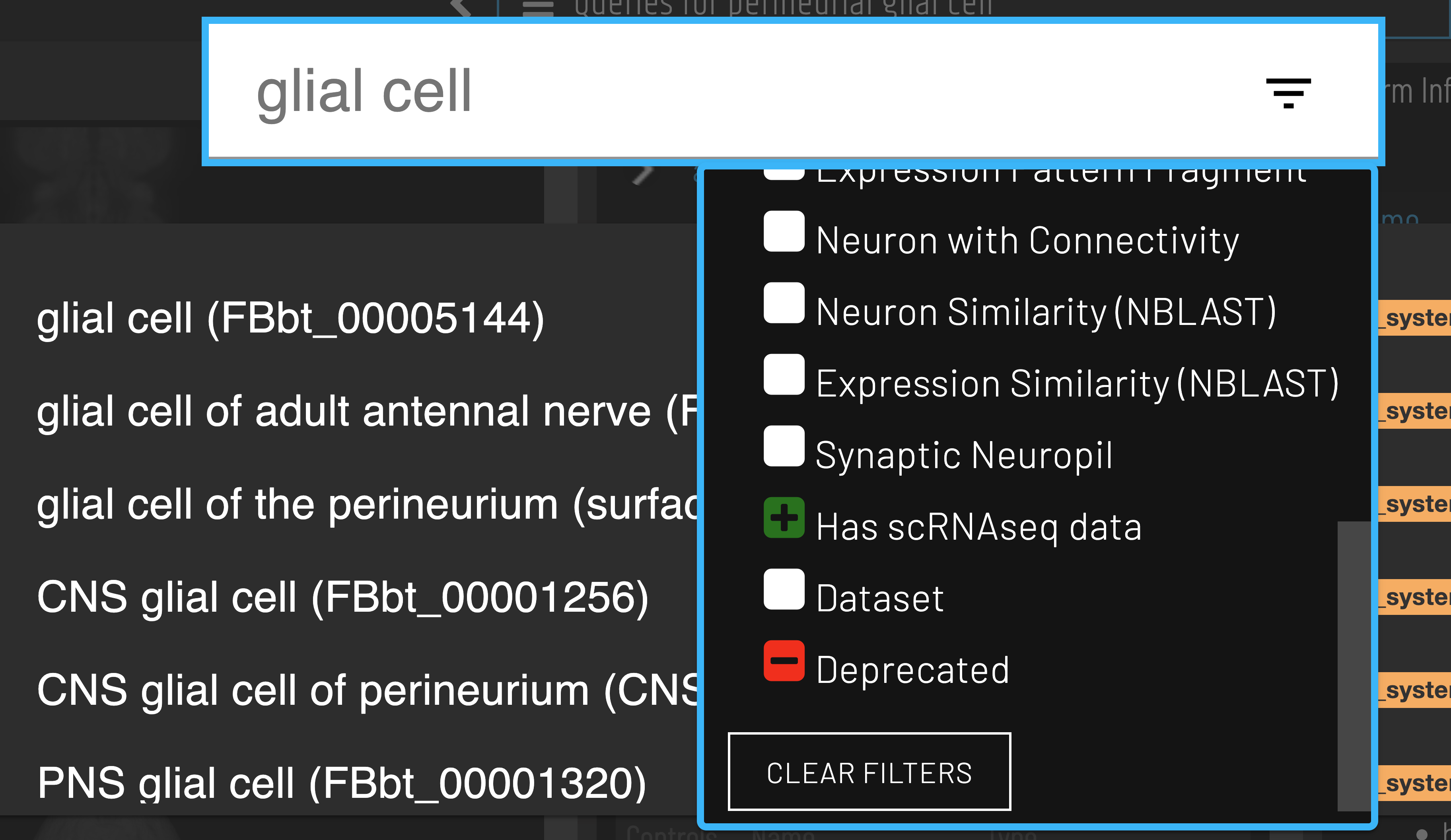
Clusters for a cell type of interest can be found via the ‘Single cell transcriptomics data for…’ query.

Gene expression data

After selecting a cluster, gene expression can be retrieved via the ‘Genes expressed in…’ query.

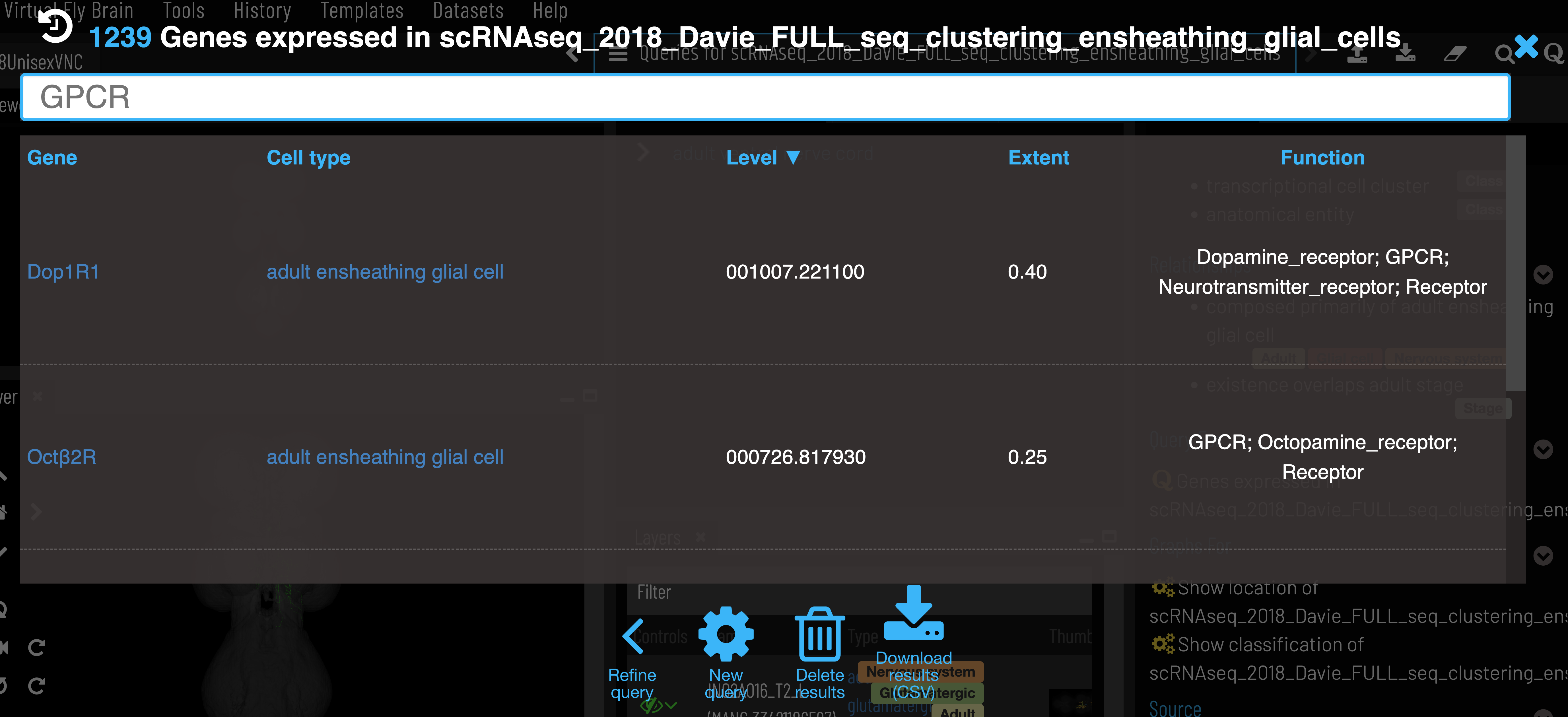
Expression level is the mean counts per million reads of all cells in the cell type cluster that express the given gene. Expression extent is the proportion of cells within the cluster that express the given gene. VFB only shows genes that are expressed in at least 20% of cells in the cluster (Extent > 0.2).

Gene semantic tags

We add semantic tags to genes to allow quick searching and filtering of results (‘Function’ column of gene expression data). These tags are based on FlyBase Gene Group membership and GO annotations, which are all sourced from FlyBase. A full list of gene tags with their associated Gene group and GO terms can be found here.

API

Data can also be retrieved using VFB_connect.

Tutorial

Documentation

Data sources and processing

1. Raw scRNAseq data is ingested by the EBI Single Cell Expression Atlas (SCEA). Where possible, cells are linked to cell types from the Drosophila Anatomy Ontology based on author annotations. Data is reprocessed, filtered and reclustered.
2. FlyBase takes data from EBI, keeping only cells that are linked to ontology terms and generating summary expression data for each cell type (cluster).
3. VFB takes control/wild type expression data from FlyBase for datasets where at least one nervous system cell type is present and filter out any genes expressed in less than 20% of cells per cluster.

Database schema

A simplified schema showing how scRNAseq data is stored in the VFB Neo4j database is shown below:

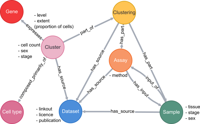
Cell types are classes from the Drosophila Anatomy Ontology and are also linked to several other types of data in VFB, such as images, connectomics and driver expression information.

3 - Application Programming Interface (API) Tutorials

3.1 - VFB connect API overview

VFB connect API overview

The VFB connect API provides programmatic access to the databases underlying Virtual Fly Brain.

At the core of Virtual Fly Brain is a set of curated terms for Drosophila neuro-anatomy organised into a queryable classification, including terms for brain regions, e.g. nodulus and neurons e.g. MBON01. These terms are used to annotate and classify individual brain regions and neurons in images and connectomics data. For example the term MBON01 is used to classify individual neurons from sources including the CATMAID-FAFB and Neuprint-HemiBrain databases. VFB stores both registered 3D images and connectomics data (where available) for all of these neurons.

A single VfbConnect object wraps database connections and canned queries against all open VFB databases. It includes methods for retreiving metadata about anatomy, individual brain regions and neurons including IDs for these that can be used for queries against other databases (e.g. CATMAID & neuprint). It provides methods for downloading images and connectomics data. It provides access to sophisticated queries for anatomical classes and individual neurons according to their classification & properties.

Locations for methods under a VfbConnect object.

1. Under vc.neo_query_wrapper are
   1. A set of methods that take lists of IDs as a primary argument and return metadata.
   2. A set of methods for mapping between VFB IDs and external IDs
2. Directly under vc are:
   1. A set of methods that take the names of classes in VFB e.g. ’nodulus’ or ‘Kenyon cell’, or simple query expressions using the names of classes and return metadata about the classes.
   2. A set methods for querying connectivity and similarity
3. Direct access to API queries is provided under the ’nc’ and ‘oc’ attributes for Neo4J and OWL queries respectively. We will not cover details of how to use these here.

Note: available methods and their documentation are easy to explore in DeepNote. Tab completion and type adhead can be used to help find methods. Float your cursor over a method to see its signature and docstring.

1. vc.neo_query_wrapper methods overview

1.1 vc.neo_query_wrapper TermInfo queries return the results of a VFB Term Information window as JSON, following the VFB_JSON standard, or a summary that can easily be converted into a DataFrame.

# A query for full TermInfo.  This probably produces more information than you will need for most purposes.

vc.neo_query_wrapper.get_type_TermInfo(['FBbt_00003686'])

    [{'term': {'core': {'iri': 'http://purl.obolibrary.org/obo/FBbt_00003686',
        'symbol': '',
        'types': ['Entity',
         'Anatomy',
         'Nervous_system',
         'Cell',
         'Neuron',
         'Class'],
        'label': 'Kenyon cell',
        'short_form': 'FBbt_00003686'},
       'description': ['Intrinsic neuron of the mushroom body. They have tightly-packed cell bodies, situated in the rind above the calyx of the mushroom body (Ito et al., 1997). Four short fascicles, one per lineage, extend from the cell bodies of the Kenyon cells into the calyx (Ito et al., 1997). These 4 smaller fascicles converge in the calyx where they arborize and form pre- and post-synaptic terminals (Christiansen et al., 2011), with different Kenyon cells receiving input in different calyx regions/accessory calyces (Tanaka et al., 2008). They emerge from the calyx as a thick axon bundle referred to as the peduncle that bifurcates to innervate the dorsal and medial lobes of the mushroom body (Tanaka et al., 2008).'],
       'comment': ['Pre-synaptic terminals were identified using two presynaptic markers (Brp and Dsyd-1) and post-synaptic terminals by labelling a subunit of the acetylcholine receptor (Dalpha7) in genetically labelled Kenyon cells (Christiansen et al., 2011).']},
      'query': 'Get JSON for Class',
      'version': '44725ae',
      'parents': [{'iri': 'http://purl.obolibrary.org/obo/FBbt_00001366',
        'symbol': '',
        'types': ['Entity',
         'Anatomy',
         'Nervous_system',
         'Cell',
         'Neuron',
         'Class'],
        'label': 'supraesophageal ganglion neuron',
        'short_form': 'FBbt_00001366'},
       {'iri': 'http://purl.obolibrary.org/obo/FBbt_00007484',
        'symbol': '',
        'types': ['Entity',
         'Anatomy',
         'Nervous_system',
         'Cell',
         'Neuron',
         'Class'],
        'label': 'mushroom body intrinsic neuron',
        'short_form': 'FBbt_00007484'}],
      'relationships': [{'relation': {'type': 'develops_from',
         'iri': 'http://purl.obolibrary.org/obo/RO_0002202',
         'label': 'develops from'},
        'object': {'iri': 'http://purl.obolibrary.org/obo/FBbt_00007113',
         'symbol': '',
         'types': ['Entity',
          'Anatomy',
          'Nervous_system',
          'Cell',
          'Neuroblast',
          'Class'],
         'label': 'mushroom body neuroblast',
         'short_form': 'FBbt_00007113'}},
       {'relation': {'type': 'overlaps',
         'iri': 'http://purl.obolibrary.org/obo/RO_0002131',
         'label': 'overlaps'},
        'object': {'iri': 'http://purl.obolibrary.org/obo/FBbt_00003687',
         'symbol': '',
         'types': ['Entity',
          'Synaptic_neuropil',
          'Anatomy',
          'Nervous_system',
          'Synaptic_neuropil_domain',
          'Class'],
         'label': 'mushroom body pedunculus',
         'short_form': 'FBbt_00003687'}},
       {'relation': {'type': 'part_of',
         'iri': 'http://purl.obolibrary.org/obo/BFO_0000050',
         'label': 'is part of'},
        'object': {'iri': 'http://purl.obolibrary.org/obo/FBbt_00005801',
         'symbol': '',
         'types': ['Entity',
          'Synaptic_neuropil',
          'Anatomy',
          'Nervous_system',
          'Synaptic_neuropil_block',
          'Class'],
         'label': 'mushroom body',
         'short_form': 'FBbt_00005801'}},
       {'relation': {'type': 'receives_synaptic_input_in',
         'iri': 'http://purl.obolibrary.org/obo/RO_0013002',
         'label': 'receives synaptic input in'},
        'object': {'iri': 'http://purl.obolibrary.org/obo/FBbt_00003685',
         'symbol': '',
         'types': ['Entity',
          'Synaptic_neuropil',
          'Anatomy',
          'Nervous_system',
          'Synaptic_neuropil_domain',
          'Class'],
         'label': 'mushroom body calyx',
         'short_form': 'FBbt_00003685'}}],
      'xrefs': [],
      'anatomy_channel_image': [{'channel_image': {'channel': {'iri': 'http://virtualflybrain.org/reports/VFBc_jrchjwig',
          'symbol': '',
          'types': ['Entity', 'Individual'],
          'label': 'KCg-t_R - 5812981989_c',
          'short_form': 'VFBc_jrchjwig'},
         'image': {'template_channel': {'iri': 'http://virtualflybrain.org/reports/VFBc_00101567',
           'symbol': '',
           'types': ['Entity', 'Individual', 'Template'],
           'label': 'JRC2018Unisex_c',
           'short_form': 'VFBc_00101567'},
          'index': [],
          'template_anatomy': {'iri': 'http://virtualflybrain.org/reports/VFB_00101567',
           'symbol': '',
           'types': ['Entity',
            'has_image',
            'Adult',
            'Anatomy',
            'Nervous_system',
            'Individual',
            'Template'],
           'label': 'JRC2018Unisex',
           'short_form': 'VFB_00101567'},
          'image_folder': 'http://www.virtualflybrain.org/data/VFB/i/jrch/jwig/VFB_00101567/'},
         'imaging_technique': {'iri': 'http://purl.obolibrary.org/obo/FBbi_00050000',
          'symbol': 'FIB-SEM',
          'types': ['Entity', 'Class'],
          'label': 'focussed ion beam scanning electron microscopy (FIB-SEM)',
          'short_form': 'FBbi_00050000'}},
        'anatomy': {'iri': 'http://virtualflybrain.org/reports/VFB_jrchjwig',
         'symbol': '',
         'types': ['Entity',
          'has_image',
          'Adult',
          'Anatomy',
          'has_neuron_connectivity',
          'Cell',
          'Individual',
          'has_region_connectivity',
          'NBLAST',
          'Nervous_system',
          'Neuron'],
         'label': 'KCg-t_R - 5812981989',
         'short_form': 'VFB_jrchjwig'}},
       {'channel_image': {'channel': {'iri': 'http://virtualflybrain.org/reports/VFBc_jrchjwig',
          'symbol': '',
          'types': ['Entity', 'Individual'],
          'label': 'KCg-t_R - 5812981989_c',
          'short_form': 'VFBc_jrchjwig'},
         'image': {'template_channel': {'iri': 'http://virtualflybrain.org/reports/VFBc_00101384',
           'symbol': '',
           'types': ['Entity', 'Individual', 'Template'],
           'label': 'JRC_FlyEM_Hemibrain_c',
           'short_form': 'VFBc_00101384'},
          'index': [],
          'template_anatomy': {'iri': 'http://virtualflybrain.org/reports/VFB_00101384',
           'symbol': '',
           'types': ['Entity',
            'has_image',
            'Adult',
            'Anatomy',
            'Nervous_system',
            'Individual',
            'Template'],
           'label': 'JRC_FlyEM_Hemibrain',
           'short_form': 'VFB_00101384'},
          'image_folder': 'http://www.virtualflybrain.org/data/VFB/i/jrch/jwig/VFB_00101384/'},
         'imaging_technique': {'iri': 'http://purl.obolibrary.org/obo/FBbi_00050000',
          'symbol': 'FIB-SEM',
          'types': ['Entity', 'Class'],
          'label': 'focussed ion beam scanning electron microscopy (FIB-SEM)',
          'short_form': 'FBbi_00050000'}},
        'anatomy': {'iri': 'http://virtualflybrain.org/reports/VFB_jrchjwig',
         'symbol': '',
         'types': ['Entity',
          'has_image',
          'Adult',
          'Anatomy',
          'has_neuron_connectivity',
          'Cell',
          'Individual',
          'has_region_connectivity',
          'NBLAST',
          'Nervous_system',
          'Neuron'],
         'label': 'KCg-t_R - 5812981989',
         'short_form': 'VFB_jrchjwig'}},
       {'channel_image': {'channel': {'iri': 'http://virtualflybrain.org/reports/VFBc_jrchjwih',
          'symbol': '',
          'types': ['Entity', 'Individual'],
          'label': 'KCg-t_R - 1392655948_c',
          'short_form': 'VFBc_jrchjwih'},
         'image': {'template_channel': {'iri': 'http://virtualflybrain.org/reports/VFBc_00101567',
           'symbol': '',
           'types': ['Entity', 'Individual', 'Template'],
           'label': 'JRC2018Unisex_c',
           'short_form': 'VFBc_00101567'},
          'index': [],
          'template_anatomy': {'iri': 'http://virtualflybrain.org/reports/VFB_00101567',
           'symbol': '',
           'types': ['Entity',
            'has_image',
            'Adult',
            'Anatomy',
            'Nervous_system',
            'Individual',
            'Template'],
           'label': 'JRC2018Unisex',
           'short_form': 'VFB_00101567'},
          'image_folder': 'http://www.virtualflybrain.org/data/VFB/i/jrch/jwih/VFB_00101567/'},
         'imaging_technique': {'iri': 'http://purl.obolibrary.org/obo/FBbi_00050000',
          'symbol': 'FIB-SEM',
          'types': ['Entity', 'Class'],
          'label': 'focussed ion beam scanning electron microscopy (FIB-SEM)',
          'short_form': 'FBbi_00050000'}},
        'anatomy': {'iri': 'http://virtualflybrain.org/reports/VFB_jrchjwih',
         'symbol': '',
         'types': ['Entity',
          'has_image',
          'Adult',
          'Anatomy',
          'has_neuron_connectivity',
          'Cell',
          'Individual',
          'has_region_connectivity',
          'NBLAST',
          'Nervous_system',
          'Neuron'],
         'label': 'KCg-t_R - 1392655948',
         'short_form': 'VFB_jrchjwih'}},
       {'channel_image': {'channel': {'iri': 'http://virtualflybrain.org/reports/VFBc_jrchjwih',
          'symbol': '',
          'types': ['Entity', 'Individual'],
          'label': 'KCg-t_R - 1392655948_c',
          'short_form': 'VFBc_jrchjwih'},
         'image': {'template_channel': {'iri': 'http://virtualflybrain.org/reports/VFBc_00101384',
           'symbol': '',
           'types': ['Entity', 'Individual', 'Template'],
           'label': 'JRC_FlyEM_Hemibrain_c',
           'short_form': 'VFBc_00101384'},
          'index': [],
          'template_anatomy': {'iri': 'http://virtualflybrain.org/reports/VFB_00101384',
           'symbol': '',
           'types': ['Entity',
            'has_image',
            'Adult',
            'Anatomy',
            'Nervous_system',
            'Individual',
            'Template'],
           'label': 'JRC_FlyEM_Hemibrain',
           'short_form': 'VFB_00101384'},
          'image_folder': 'http://www.virtualflybrain.org/data/VFB/i/jrch/jwih/VFB_00101384/'},
         'imaging_technique': {'iri': 'http://purl.obolibrary.org/obo/FBbi_00050000',
          'symbol': 'FIB-SEM',
          'types': ['Entity', 'Class'],
          'label': 'focussed ion beam scanning electron microscopy (FIB-SEM)',
          'short_form': 'FBbi_00050000'}},
        'anatomy': {'iri': 'http://virtualflybrain.org/reports/VFB_jrchjwih',
         'symbol': '',
         'types': ['Entity',
          'has_image',
          'Adult',
          'Anatomy',
          'has_neuron_connectivity',
          'Cell',
          'Individual',
          'has_region_connectivity',
          'NBLAST',
          'Nervous_system',
          'Neuron'],
         'label': 'KCg-t_R - 1392655948',
         'short_form': 'VFB_jrchjwih'}},
       {'channel_image': {'channel': {'iri': 'http://virtualflybrain.org/reports/VFBc_jrchjwii',
          'symbol': '',
          'types': ['Entity', 'Individual'],
          'label': 'KCg-t_R - 785918963_c',
          'short_form': 'VFBc_jrchjwii'},
         'image': {'template_channel': {'iri': 'http://virtualflybrain.org/reports/VFBc_00101567',
           'symbol': '',
           'types': ['Entity', 'Individual', 'Template'],
           'label': 'JRC2018Unisex_c',
           'short_form': 'VFBc_00101567'},
          'index': [],
          'template_anatomy': {'iri': 'http://virtualflybrain.org/reports/VFB_00101567',
           'symbol': '',
           'types': ['Entity',
            'has_image',
            'Adult',
            'Anatomy',
            'Nervous_system',
            'Individual',
            'Template'],
           'label': 'JRC2018Unisex',
           'short_form': 'VFB_00101567'},
          'image_folder': 'http://www.virtualflybrain.org/data/VFB/i/jrch/jwii/VFB_00101567/'},
         'imaging_technique': {'iri': 'http://purl.obolibrary.org/obo/FBbi_00050000',
          'symbol': 'FIB-SEM',
          'types': ['Entity', 'Class'],
          'label': 'focussed ion beam scanning electron microscopy (FIB-SEM)',
          'short_form': 'FBbi_00050000'}},
        'anatomy': {'iri': 'http://virtualflybrain.org/reports/VFB_jrchjwii',
         'symbol': '',
         'types': ['Entity',
          'has_image',
          'Adult',
          'Anatomy',
          'has_neuron_connectivity',
          'Cell',
          'Individual',
          'has_region_connectivity',
          'NBLAST',
          'Nervous_system',
          'Neuron'],
         'label': 'KCg-t_R - 785918963',
         'short_form': 'VFB_jrchjwii'}}],
      'pub_syn': [{'pub': {'core': {'iri': 'http://flybase.org/reports/Unattributed',
          'symbol': '',
          'types': ['Entity', 'Individual', 'pub'],
          'label': '',
          'short_form': 'Unattributed'},
         'FlyBase': '',
         'PubMed': '',
         'DOI': ''},
        'synonym': {'type': '', 'label': 'KC', 'scope': 'has_exact_synonym'}},
       {'pub': {'core': {'iri': 'http://flybase.org/reports/FBrf0236359',
          'symbol': '',
          'types': ['Entity', 'Individual', 'pub'],
          'label': 'Eichler et al., 2017, Nature 548(7666): 175--182',
          'short_form': 'FBrf0236359'},
         'FlyBase': 'FBrf0236359',
         'PubMed': '28796202',
         'DOI': '10.1038/nature23455'},
        'synonym': {'type': '',
         'label': 'mature Kenyon cell',
         'scope': 'has_exact_synonym'}},
       {'pub': {'core': {'iri': 'http://flybase.org/reports/FBrf0111409',
          'symbol': '',
          'types': ['Entity', 'Individual', 'pub'],
          'label': 'Lee et al., 1999, Development 126(18): 4065--4076',
          'short_form': 'FBrf0111409'},
         'FlyBase': '',
         'PubMed': '10457015',
         'DOI': ''},
        'synonym': {'type': '',
         'label': 'MB neuron',
         'scope': 'has_narrow_synonym'}}],
      'def_pubs': [{'core': {'iri': 'http://flybase.org/reports/FBrf0214059',
         'symbol': '',
         'types': ['Entity', 'Individual', 'pub'],
         'label': 'Christiansen et al., 2011, J. Neurosci. 31(26): 9696--9707',
         'short_form': 'FBrf0214059'},
        'FlyBase': '',
        'PubMed': '21715635',
        'DOI': '10.1523/JNEUROSCI.6542-10.2011'},
       {'core': {'iri': 'http://flybase.org/reports/FBrf0092568',
         'symbol': '',
         'types': ['Entity', 'Individual', 'pub'],
         'label': 'Ito et al., 1997, Development 124(4): 761--771',
         'short_form': 'FBrf0092568'},
        'FlyBase': '',
        'PubMed': '9043058',
        'DOI': ''},
       {'core': {'iri': 'http://flybase.org/reports/FBrf0205263',
         'symbol': '',
         'types': ['Entity', 'Individual', 'pub'],
         'label': 'Tanaka et al., 2008, J. Comp. Neurol. 508(5): 711--755',
         'short_form': 'FBrf0205263'},
        'FlyBase': '',
        'PubMed': '18395827',
        'DOI': '10.1002/cne.21692'}]}]

# A query for summary info
import pandas as pd

summary = vc.neo_query_wrapper.get_type_TermInfo(['FBbt_00003686'], summary=True)
summary_tab = pd.DataFrame.from_records(summary)
summary_tab

# A different method is needed to get info about individual neurons

summary = vc.neo_query_wrapper.get_anatomical_individual_TermInfo(['VFB_jrchjrch'], summary=True)
summary_tab = pd.DataFrame.from_records(summary)
summary_tab

1.2 The neo_query_wrapper also includes methods for mapping between IDs from different sources.

# Some bodyIDs of HemiBrain neurons from the neuprint DataBase:
bodyIDs = [1068958652, 571424748, 1141631198]
vc.neo_query_wrapper.xref_2_vfb_id(map(str, bodyIDs)) # Note IDs must be strings

    {'1068958652': [{'db': 'neuronbridge', 'vfb_id': 'VFB_jrchjwda'},
      {'db': 'neuronbridge', 'vfb_id': 'VFB_jrch06r9'},
      {'db': 'neuprint_JRC_Hemibrain_1point0point1', 'vfb_id': 'VFB_jrch06r9'},
      {'db': 'neuprint_JRC_Hemibrain_1point1', 'vfb_id': 'VFB_jrchjwda'}],
     '571424748': [{'db': 'neuronbridge', 'vfb_id': 'VFB_jrch06r6'},
      {'db': 'neuronbridge', 'vfb_id': 'VFB_jrchjwct'},
      {'db': 'neuprint_JRC_Hemibrain_1point0point1', 'vfb_id': 'VFB_jrch06r6'},
      {'db': 'neuprint_JRC_Hemibrain_1point1', 'vfb_id': 'VFB_jrchjwct'}],
     '1141631198': [{'db': 'neuronbridge', 'vfb_id': 'VFB_jrch05uz'},
      {'db': 'neuronbridge', 'vfb_id': 'VFB_jrchjw8r'},
      {'db': 'neuprint_JRC_Hemibrain_1point0point1', 'vfb_id': 'VFB_jrch05uz'},
      {'db': 'neuprint_JRC_Hemibrain_1point1', 'vfb_id': 'VFB_jrchjw8r'}]}

# xref queries can be constrained by DB. Results can optionally be reversed

vc.neo_query_wrapper.xref_2_vfb_id(map(str, bodyIDs), db = 'neuprint_JRC_Hemibrain_1point1' , reverse_return=True)

    {'VFB_jrchjw8r': [{'acc': '1141631198',
       'db': 'neuprint_JRC_Hemibrain_1point1'}],
     'VFB_jrchjwct': [{'acc': '571424748',
       'db': 'neuprint_JRC_Hemibrain_1point1'}],
     'VFB_jrchjwda': [{'acc': '1068958652',
       'db': 'neuprint_JRC_Hemibrain_1point1'}]}

2. vc direct methods overview

2.1 Methods that take the names of classes in VFB e.g. ’nodulus’ or ‘Kenyon cell’, or simple query expressions using the names of classes and return metadata about the classes or individual neurons.

KC_types = vc.get_subclasses("Kenyon cell", summary=True)
pd.DataFrame.from_records(KC_types)

    Running query: FBbt:00003686
    Query URL: http://owl.virtualflybrain.org/kbs/vfb/subclasses?object=FBbt%3A00003686&prefixes=%7B%22FBbt%22%3A+%22http%3A%2F%2Fpurl.obolibrary.org%2Fobo%2FFBbt_%22%2C+%22RO%22%3A+%22http%3A%2F%2Fpurl.obolibrary.org%2Fobo%2FRO_%22%2C+%22BFO%22%3A+%22http%3A%2F%2Fpurl.obolibrary.org%2Fobo%2FBFO_%22%7D&direct=False
    Query results: 37

2.2 Methods for querying connectivity

Please see Connectivity Notebook for examples.

3.2 - Guide to Working with Images from Virtual Fly Brain (VFB) Using the VFBConnect Library

Prerequisites

Before starting, ensure you have the VFBConnect library installed. The recommended Python version is 3.10.14, as this version is tested against the library.

pip install vfb-connect

Importing the VFBConnect Library

Start by importing the VFBConnect library. This library provides a simple interface to interact with neuron data from the Virtual Fly Brain.

from vfb_connect import vfb

Retrieving Neuron Data

To work with specific neurons, you can use the vfb.term() function. This function takes a unique identifier (e.g., ID, label, synonym) for the neuron.

Example: Retrieving a Single Neuron

neuron = vfb.term('5th s-LNv (FlyEM-HB:511051477)')

The neuron variable now holds data about the neuron identified by the given term.

Working with Neuron Data

The retrieved neuron object can provide different representations of neuron data, such as its skeleton, mesh, and volume. These representations can be visualized using various plotting methods.

# Access the skeleton representation
neuron_skeleton = neuron.skeleton

# Check the type of the skeleton representation
print(type(neuron_skeleton))  # Output: <class 'navis.neuron.Neuron'>

# Plot the skeleton in 2D
neuron_skeleton.plot2d()

# Access the mesh representation
neuron_mesh = neuron.mesh

# Access the volume representation
neuron_volume = neuron.volume

Retrieving Multiple Neurons

You can retrieve multiple neurons using the vfb.terms() function, which accepts a list of neuron identifiers.

Example: Retrieving Multiple Neurons

neurons = vfb.terms(['5th s-LNv', 'fru-M-300008', 'catmaid_fafb:8876600'])

This command retrieves multiple neurons, which can then be visualized or manipulated collectively.

Flexible Matching Capabilities

One of the key features of the VFBConnect library is its flexible matching capability. The vfb.terms() function can accept a variety of identifiers, such as:

• IDs: Unique identifiers assigned to each neuron.
• Xref (Cross-references): External references that relate to other datasets.
• Labels: Human-readable names for neurons.
• Symbols: Abbreviated names or symbols used to represent neurons.
• Synonyms: Alternative names by which a neuron might be known.
• Partial Matching: You can provide a partial name, and VFBConnect will attempt to find the best match.
• Case Insensitive Matching: Matching is case insensitive, so if an exact match isn’t found, ‘5th s-LNv’ and ‘5TH S-LNV’ are treated the same. This allows for more flexible querying without worrying about exact case matching.

Example: Using Flexible Matching

neurons = vfb.terms('5th s-LN')

If an exact match isn’t found, VFBConnect will provide potential matches. This feature ensures that even with partial or approximate information, you can still retrieve the relevant neuron data.

Output Example:

Notice: No exact match found, but potential matches starting with '5th s-LN': 
'5th s-LNv (FlyEM-HB:511051477)': 'VFB_jrchk8e0', 
'5th s-LNv': 'VFB_jrchk8e0'

This notice will help you identify the correct neuron based on the closest matches.

Visualizing Neurons

VFBConnect provides various methods to visualize neuron data, both individually and collectively.

3D Visualization

To plot neurons in 3D, use the plot3d() method. This is useful for visualizing the spatial structure of neurons.

neurons.plot3d()

2D Visualization

For 2D visualization, use the plot2d() method.

neurons.plot2d()

Viewing Merged Templates

VFBConnect also allows viewing merged templates of neurons, combining multiple neuron structures into a single view.

neurons.show()

Opening Neurons in VFB

To open the neurons directly in Virtual Fly Brain, use the open() method. This will launch a browser window displaying the neurons in the VFB interface.

neurons.open()

Summary

• Use vfb.term() to retrieve single neuron data.
• Use vfb.terms() to retrieve multiple neurons with support for partial, case-insensitive, and flexible matching (IDs, labels, symbols, synonyms, etc.).
• Access different data representations (skeleton, mesh, volume) via neuron objects.
• Visualize neuron data in 2D and 3D.
• Use the show() method to view merged neuron templates.
• Open neuron data directly in Virtual Fly Brain with the open() method.

These examples provide a foundation for working with neuron data from Virtual Fly Brain using the VFBConnect library. By exploring different neuron representations and visualization methods, you can analyze and understand neuron structures more effectively.

3.3 - Downloading Images from VFB Using VFBconnect

Introduction

VFBconnect is a Python package that provides an interface to the Virtual Fly Brain (VFB) API. It allows users to query the VFB database and download data, including images.

Installation

Before you can use VFBconnect, you need to install it. You can do this using pip:

pip install vfb-connect

Downloading Images

To download images from VFB using VFBconnect, you need to first import the package and create a client:

from vfb_connect.cross_server_tools import VfbConnect
vc = VfbConnect()

Next, you can use the get_images method to download images. This method requires the dataset ID as an argument:

dataset_id = 'your_dataset_id'
images = vc.get_images(dataset_id)

This will return a list of images from the specified dataset. Each image is represented as a dictionary with information such as the image ID, title, and URL.

To download the images, you can loop through the list and use the urlretrieve function from the urllib.request module:

import urllib.request

for image in images:
    url = image['image_url']
    filename = image['image_id'] + '.jpg'
    urllib.request.urlretrieve(url, filename)

This will download each image and save it as a JPEG file in the current directory. The filename is the image ID.

Conclusion

This guide showed you how to use VFBconnect to download images from the Virtual Fly Brain based on a dataset. With VFBconnect, you can easily access and download data from VFB for your research.

3.4 - Programmatic search using SOLR

SOLR python example

an example using pysolr:

install:

pip install vfb-connect pysolr

example looking for label/name match:

import pysolr

solr = pysolr.Solr('https://solr.virtualflybrain.org/solr/ontology/')

term = 'medulla'

results = solr.search('label:"' + term + '"')

print(results.docs[0])

{'iri': ['http://purl.obolibrary.org/obo/FBbt_00003748'],
 'obo_id_autosuggest': ['FBbt_00003748', 'FBbt:00003748', 'FBbt 00003748'],
 'label_autosuggest': ['medulla', 'medulla', 'medulla'],
 'synonym_autosuggest': ['ME', 'Med', 'optic medulla', 'm'],
 'label': 'medulla',
 'synonym': ['ME', 'Med', 'optic medulla', 'm'],
 'short_form': 'FBbt_00003748',
 'autosuggest': ['medulla', 'ME', 'Med', 'optic medulla', 'm'],
 'facets_annotation': ['Entity',
  'Adult',
  'Anatomy',
  'Class',
  'Nervous_system',
  'Synaptic_neuropil',
  'Synaptic_neuropil_domain'],
 'unique_facets': ['Nervous_system', 'Adult', 'Synaptic_neuropil_domain'],
 'id': 'http://purl.obolibrary.org/obo/FBbt_00003748',
 'shortform_autosuggest': ['FBbt_00003748', 'FBbt:00003748', 'FBbt 00003748'],
 'obo_id': ['FBbt:00003748'],
 '_version_': 1734360220689235970}

Note: any of the above fields can be searched (autosuggest being a combination of both label and synonyms)

3.5 - Exploring Neurons in Navis

Overview

navis is a Python package for analysing, manipulating and visualizing neurons. Official documentation here.

Basic datatypes: neurons and neuron lists

navis knows three types of neurons:

1. TreeNeurons = skeletons, e.g. from CATMAID
2. MeshNeurons = meshes, e.g. from the hemibrain segmentation
3. Dotprops = points + tangent vectors (typically only used for NBLAST)

Collections of neurons are typically held in a specialized container: a NeuronList.

Neurons

In this notebook we will focus on skeletons - a.k.a. TreeNeurons - since this is what you get out of CATMAID. Let’s kick things off by having a look at what neurons look like once it’s loaded:

import navis

# Load one of the example neurons shipped with navis
# (these are olfactory projection neurons from the hemibrain data set)
n = navis.example_neurons(1, kind='skeleton')

# Print some basic info
n

WARNING: Could not load OpenGL library.

Above summary lists a couple of (computed) properties of the neuron. Each of those can also be accessed directly like so:

n.id

1734350788

There are many more properties that you might find interesting! Typing n. and pressing TAB should give auto-complete suggestions of available properties and methods. If your notebook editor has problems with that, you can fall back to using dir().

Here is an (incomplete) list of some of the more relevant properties:

• bbox: bounding box of the neuron
• cable_length: cable length
• id: every neuron has an ID
• nodes: the SWC node table underlying the neuron

And some class methods:

• reroot: reroot neuron
• plot2d/plot3d: plot the neuron (see also plotting turorial)
• copy: make and return a copy
• prune_twigs: remove small terminal twigs

As an example: this is how you get the ID of this neuron’s root node.

# Current root node of this neuron
n.root

array([1], dtype=int32)

Some of the properties such as .root or .ends are computed on-the-fly from the underlying raw data. For TreeNeurons that’s the node table (and its graph representation). The node table is a pandas DataFrame that looks effectively like a SWC:

# `.head()` gives us the first couple rows
n.nodes.head()

The methods (such as .reroot) are short-hands for main navis functions:

# Reroot neuron to another node
n2 = n.reroot(new_root=2)
# Print the new root -> expect "2"
n2.root

array([2])

# Instead of calling the shorthand method, we can also do this
n3 = navis.reroot_neuron(n, new_root=2)
n3.root

array([2])

NeuronLists

In practice you will likely work with multiple neurons at a time. For that, navis has a convenient container: NeuronLists

# Get more than one example neuron
nl = navis.example_neurons(5)

# `nl` is a NeuronList 
type(nl)

navis.core.neuronlist.NeuronList

# You can also create neuron lists yourself
my_nl = navis.NeuronList(n)

In many ways NeuronLists work like Python-lists with a couple of extras:

# Calling just the neuronlist produces a summary 
nl

# Get a single neuron from the neuronlist
nl[1]

neuronlists also support fancy indexing similar to numpy arrays:

# Get multiple neurons from the neuronlist
nl[[1, 2]]

# Slicing is also supported
nl[1:3]

Strings will be matched against the neurons’ names.

# Get neuron(s) by their name
nl['754534424']

neuronlists have a special .idx indexer that let’s you select neurons by their ID

# Get neuron(s) by their ID 
# -> note that for example neurons name == id 
nl.idx[[754534424, 722817260]]

# Access properties across neurons -> returns numpy arrays
nl.n_nodes 

array([4465, 4845, 4336, 4702, 4890])

# Select neurons by given property
# -> this works with any boolean array 
nl[nl.n_nodes >= 4500]

Exercises:

1. Select the first and the last neuron in the neuronlist
2. Select all neurons with a soma
3. Select all neurons with a soma and less than 300,000 cable length

Further reading: https://navis.readthedocs.io/en/latest/source/tutorials/neurons_intro.html

3.6 - Plotting Neurons with Navis

Plotting

navis lets you plot neurons in 2D using matplotlib (nice for figures), and in 3D using either plotly when in a notebook environment like Deepnote or using a vispy-based 3D viewer when using a Python terminal.

import navis

# This is relevant because Deepnote does not (yet) support fancy progress bars
navis.set_pbars(jupyter=False)

# Load one of the example neurons shipped with navis
n = navis.example_neurons(1, kind='skeleton')

WARNING: Could not load OpenGL library.

# Make a 2d plot 
fig, ax = navis.plot2d(n)

# Note that this is equivalent to 
# fig, ax = n.plot2d()

If you have seen an olfactory projection neuron before, you might have noticed that this neuron is upside-down. That’s because hemibrain neurons have an odd orienation in that the anterior-posterior axis is not the z- but the y-axis (they were imaged from above).

For us that just means we have to turn the camera ourselves if we want a frontal view:

# Make a 2d plot 
fig, ax = navis.plot2d(n)

# Change camera (azimuth + elevation)
ax.azim, ax.elev = -90, -90

Let’s do the same in 3d:

# Get a list of neurons
nl = navis.example_neurons(5)

# Plot
navis.plot3d(nl, width=1000)

Navigation:

• left click and drag to rotate (select “Orbital rotation” above the legend to make your life easier)
• mousewheel to zoom
• middle-mouse + drag to translate
• click legend items (single or double) to hide/unhide

Above plots are very basic examples but there are a ton of ways to tweak things to your liking. For a full list of parameters check out the docs for plot2d and plot3d.

Let’s for example change the colors. In general, colors can be:

• a string - e.g. "red" or just "r"
• an rgb/rgba tuple - e.g. (1, 0, 0) for red

# Plot all neurons in red
fig, ax = navis.plot2d(n, color='r')
ax.azim, ax.elev = -90, -90

# Plot all neurons in red (color as tuple)
fig, ax = navis.plot2d(n, color=(1, 0, 0, 1))
ax.azim, ax.elev = -90, -90

When plotting multiple neurons you can either use:

• a single color ("r" or (1, 0, 0)) -> assigned to all neurons
• a list of colors (['r', 'yellow', (0, 0, 1)]) with a color for each neuron
• a dictionary mapping neuron IDs to colors ({1734350788: 'r', 1734350908: (1, 0, 1)})
• the name of a matplotlib or seaborn color palette

# Plot with a specific color palette
navis.plot3d(nl, color='jet')

Exercises:

1. Assign rainbow colors - "red", "orange", "yellow", "green" and "blue" - as list
2. Use a dictionary to make neurons 1734350788 and 1734350908 green, and neurons 722817260, 754534424 and 754538881 red

Volumes

plot2d and plot3d also let you plot meshes. Internally these are represented as navis.Volumes (a subclass of trimesh.Trimesh):

# navis ships with a neuropil volume (in hemibrain space)
vol = navis.example_volume('neuropil')
vol

<navis.Volume(name=neuropil, color=(0.85, 0.85, 0.85, 0.2), vertices.shape=(8997, 3), faces.shape=(18000, 3))>

To plot, simply pass it to the respective plotting function:

navis.plot3d([nl, vol])

Under the hood, Volumes are treated a bit differently from neurons. So if you want to change the color, you need to do so on the object:

# Give the neuropil a reddish color
vol.color = (1, .8, .8, .4)

navis.plot3d([nl, vol], width=800)

Scatter plots

Because scatter plots are a common way of visualizing 3D data, both plot2d and plot3d provide a quick interface: (N, 3) numpy arrays and pandas.DataFrames with x, y, and z columns are interpreted as data for a scatter plot:

# Get all branch points from the node table
bp = n.branch_points
bp.head()

# Since `bp` contains x/y/z columns, we can pass it directly to the plotting functions 
navis.plot3d([n, bp],
             c='k',  # make the neuron black 
             scatter_kws=dict(color='r')  # make the markers red
             )

Fine-tuning figures

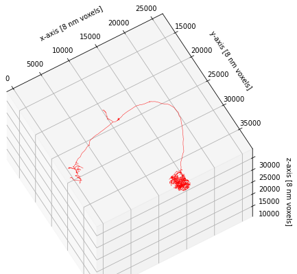
plot2d and plot3d provide a high-level interface to get your neurons on/in a matplotlib or a plotly figure, respectively. You can always use lower-level matplotlib/plotly interfaces directly to add more data or manipulate the figure. Just a cheap example:

# Plot neuron on a matplotlib figure
fig, ax = navis.plot2d(n, color='r')

# Show the neuron at a slight angle
ax.azim, ax.elev = -60, -60

# Zoom out a bit more
ax.dist = 8  # default is 7

# Unhide axes 
ax.set_axis_on()

# Label the axes
ax.set_xlabel('x-axis [8 nm voxels]')
ax.set_ylabel('y-axis [8 nm voxels]')
ax.set_zlabel('z-axis [8 nm voxels]')

Text(0.5, 0, 'z-axis [8 nm voxels]')

This concludes this brief introduction to plotting but just to note that plot2d and plot3d have a lot of additional functionality to customize the way neurons are plotted. If you have time on your hands, I recommend you check out and play around with the available parameters (e.g. linewidth, color_by, shade_by, linestyle).

3.7 - pymaid

Overview

pymaid lets you interface with a CATMAID server. It’s built on top of navis and returns data (neurons, volumes) in a way that you can plug them straight into navis to use features such as plotting.

Official documentation here.

Connecting

The VFB CATMAID servers (see here for what’s available) are public and don’t require an API token for read-only access which makes connecting simple:

import pymaid
import navis

navis.set_pbars(jupyter=False)
pymaid.set_pbars(jupyter=False)

# Connect to the VFB CATMAID server hosting the FAFB data
rm = pymaid.connect_catmaid(server="https://fafb.catmaid.virtualflybrain.org/", api_token=None, max_threads=10)

# Test call to see if connection works 
print(f'Server is running CATMAID version {rm.catmaid_version}')

WARNING: Could not load OpenGL library.
INFO  : Global CATMAID instance set. Caching is ON. (pymaid)
Server is running CATMAID version 2020.02.15-905-g93a969b37

Retrieving neurons

Let’s start with pulling a neuron based on its ID:

# Find a neuron from its ID (16) -> this is an olfactory projection neuron
n = pymaid.get_neurons(16)
n

This neuron’s type is pymaid.CatmaidNeuron, which is a subclass of navis.TreeNeuron. The list version is pymaid.CatmaidNeuronList, which a subclass of navis.NeuronList. This adds a bit of extra functionality (such as lazy loading of data) and allows CatmaidNeuron and CatmaidNeuronList work as drop in replacements for their parent classes.

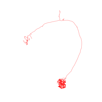
# Plot CatmaidNeuron with navis
navis.plot3d(n, width=1000, connectors=True, c='k')

get_neurons() returns neurons including their “connectors” - i.e. pre- (red) and postsynapses (blue). For this particular neuron, the published data comprehensively labels the axonal synapses but not the dendrites. Analogous to the nodes table, you can access the connectors like so:

n.connectors.head()

Let’s run a bigger example and pull all data published with Bates, Schlegel et al. 2020. For this, we will use “annotations”. These are effectively text labels that group neurons together, in this case by paper. Instead of get_neurons we can use find_neurons to avoid downloading unnecessary data.

bates = pymaid.find_neurons(annotations='Paper: Bates and Schlegel et al 2020')
len(bates)

INFO  : Found 583 neurons matching the search parameters (pymaid)





583

bates is a CatmaidNeuronList containing 583 neurons. Importantly pymaid has not yet loaded any data other than names! Note all the “NAs” in the summary:

bates.head()

We could have used pymaid.get_neurons(annotations='Paper: Bates and Schlegel et al 2020') instead to load all data up-front, but this would increase memory usage.

The CatmaidNeuronList we have created will lazy load data from the server when required.

# Access the first neuron's nodes 
# -> this will trigger a data download
_ = bates[0].nodes 

# Run summary again 
bates.head()

We have now loaded data for the first neuron.

Next we willl find and plot all uniglomelar DA1 projection neurons by their name.

# Name will be match pattern "Uniglomerular {tract} DA1 {lineage}"
import re 
prog = re.compile("Uniglomerular(.*?) DA1 ")

# Match all neuron names in `bates` against that pattern
is_da1 = list(map(lambda x: prog.match(x) != None, bates.name))

# Subset list 
da1 = bates[is_da1]
da1.head()

# Plot neurons by their lineage  
for n in da1:
    # Split name into components and keep the lineage
    n.lineage = n.name.split(' ')[3]    

# Generate a color per lineage
import seaborn as sns
import numpy as np 

lineages = np.unique(da1.lineage) 
lin_cmap = dict(zip(lineages, sns.color_palette('muted', len(lineages))))
neuron_cmap = {n.id: lin_cmap[n.lineage] for n in da1}

navis.plot3d(da1, color=neuron_cmap, hover_name=True)

Let’s add the neuropil meshes. These are called “volumes” on the CATMAID servers. To find out what’s available:

vols = pymaid.get_volume()
vols.head()

INFO  : Retrieving list of available volumes. (pymaid)

# Get the neuropil volume 
v14neuropil = pymaid.get_volume('v14.neuropil')

# Make it slightly more transparent
v14neuropil.color = (.8, .8, .8, .3)

INFO  : Cached data used. Use `pymaid.clear_cache()` to clear. (pymaid)

# Plot with neuropil volume
navis.plot3d([da1, v14neuropil], color=neuron_cmap)

Suggested exercises:

• find all uniglomerular projection neurons (name starts with Uniglomerular)
• calculate the number of pre-/post-synapses in the right lateral horn (LH) (use pymaid.get_volume and navis.in_volume)
• group the neurons by glomerulus based on label (nomenclature is Uniglomerular {tract} {glomerulus} {lineage} {metadata})
• plot LH pre- vs post-synapses in a scatter plot (e.g. using seaborn.scatterplot)

Pulling connectivity

CATMAID lets you fetch connectivity data either as a list of up- and downstream partners or as whole adjacency matrices.

# Pull downstream partners of DA1 PNs
da1_ds = pymaid.get_partners(da1,
                             threshold=3,  # anything with >= 3 synapses
                             directions=['outgoing']  # downstream partners only
                              )

# Result is a pandas DataFrame
da1_ds.head()

INFO  : Fetching connectivity table for 17 neurons (pymaid)
INFO  : Done. Found 0 pre-, 270 postsynaptic and 0 gap junction-connected neurons (pymaid)

Each row is a synaptic downstream partner of our query DA1 neurons. The columns to the left contain the synapses they receive from individual query neurons. For example 1811442 (first row) receives 30 synapses from the DA1 PN with ID 2863104.

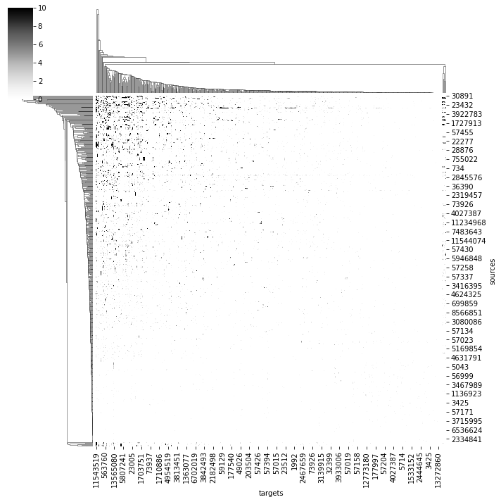
# Get an adjacency matrix between all Bates, Schlegel et al. neurons
adj = pymaid.adjacency_matrix(bates)
adj.head()

# Plot a quick & dirty adjacency matrix
import seaborn as sns 

ax = sns.clustermap(adj, vmax=10, cmap='Greys')

/shared-libs/python3.7/py/lib/python3.7/site-packages/seaborn/matrix.py:649: UserWarning:

Clustering large matrix with scipy. Installing `fastcluster` may give better performance.

We can also ask for where in space specific connections are made:

# Axo-axonic connections between two different types of DA1 PNs
cn = pymaid.get_connectors_between(2863104, 1811442)
cn.head()

# Visualize
points = np.vstack(cn.connector_loc)

navis.plot3d([da1.idx[[2863104, 1811442]],  # plot the two neurons
              points],  # plot the points of synaptic contacts as scatter 
              scatter_kws=dict(name="synaptic contacts")
              )

3.8 - NBLAST

Overview

NBLAST (Costa et al., 2016) is a method to quantify morphological similarity. It works on “dotprops” which represent neurons as tangent vectors. For each tangent vector in the query neuron, NBLAST finds the closest tangent vector in the target neuron and calculates a score from the distance between and the dotproduct of the two vectors. The final NBLAST score is the sum over all query-target vector pairs. Typically, this score is normalized to a self-self comparison (i.e. a perfect match would be 1).

Finding Matching Neurons

VFB computes NBLAST scores for all neurons in its database. So if all you want is a list of similar neurons, it’s fastest (and easiest) to get those directly from VFB.

# Import libs and initialise API objects
from vfb_connect.cross_server_tools import VfbConnect
import navis.interfaces.neuprint as neu

import pandas as pd
import navis

navis.set_pbars(jupyter=False)

vc = VfbConnect()
client = neu.Client('https://neuprint.janelia.org', dataset='hemibrain:v1.1')

First let’s write a function to grab VFB neurons and turn them into navis neurons. This is modified from vc.neo_query_wrapper.get_images.

import requests
from tqdm import tqdm

def get_vfb_neurons(vfb_ids, template='JRC2018Unisex'):
    """Load neurons from VFB as navis.TreeNeurons."""
    vfb_ids = list(navis.utils.make_iterable(vfb_ids))
    inds = vc.neo_query_wrapper.get_anatomical_individual_TermInfo(short_forms=vfb_ids)
    nl = []
    # Note: queries should be parallelized in the future 
    # -> for pymaid I use request-futures which works really well
    for i in tqdm(inds, desc='Loading VFB neurons', leave=False):        
        if not ('has_image' in i['term']['core']['types']):
            continue
        label = i['term']['core']['label']
        image_matches = [x['image'] for x in i['channel_image']]
        if not image_matches:
            continue
        for imv in image_matches:
            if imv['template_anatomy']['label'] == template:
                r = requests.get(imv['image_folder'] + '/volume.swc')
                ### Slightly dodgy warning - could mask network errors
                if not r.ok:
                    warnings.warn("No '%s' file found for '%s'." % (image_type, label))
                    continue

                # `id` should ideally be unique but that's not enforced
                n = navis.TreeNeuron(r.text, name=label, id=i['term']['core']['short_form'])   

                # This registers attributes that you want to show in the summary
                # alternatively we could have a generic attribute like so:
                # n.template = template
                n._register_attr("template", template, temporary=False)

                # I assume all available templates are in microns?
                # @Robbie -do we have this metadata on templates?  If not, we should add ASAP.
                n.units = '1 micron'

                nl.append(n)
    return navis.NeuronList(nl)

# Search for similar neurons using the VFB ID of an ellipsoid body neuron in FAFB
# We got that ID from a search on the VFB website
similar_to_EPG6L1 = vc.get_similar_neurons('VFB_001012ay')
similar_to_EPG6L1 

# Read those neurons from VFB 
query = get_vfb_neurons('VFB_001012ay')
matches = get_vfb_neurons(similar_to_EPG6L1.id.values)

matches

# Define colors such that query is black 
import seaborn as sns 
colors = ['k'] + sns.color_palette('muted', len(matches))

navis.plot3d([query, matches], color=colors)

These like a good match!

Clustering Groups of Neurons

Now imagine you have a set of neurons and you want to group them into morphologically similar “types”. To demonstrate this, we will take some ellipsoid body neurons from VFB and cluster them using NBLAST.

# Find instances of EB-PB-gall neurons
eb_pb_ids = pd.DataFrame.from_records(vc.get_instances("adult ellipsoid body-protocerebral bridge-gall neuron"))
eb_pb_ids.head()

# Get the neurons from VFB
eb_pb = get_vfb_neurons(eb_pb_ids.id.values)
eb_pb

Loading VFB neurons: 100%|██████████| 62/62 [01:04<00:00,  1.04s/it]

Now that we have the skeletons, we need to turn them into dotprops. Keep in mind that:

1. NBLAST is optimized for data in microns. Since our neurons are in the JRC2018Unisex template, they already are.
2. Neurons should have the same sampling rate (i.e. nodes per micron). To ensure this we will resample the neurons to 1 point per micron.
3. We won’t be doing this this time around but we typically simplify the neurons slightly by e.g. pruning small twigs (navis.prune_twigs()) to reduce noise.

eb_dps = navis.make_dotprops(eb_pb, resample=1, k=5)

# Note this NeuronList /contains dotprops now
eb_dps

To illustrate what dotprops are, lets visualize one side-by-side with its skeleton.

sk = eb_pb[0].copy()
dp = eb_dps[0].copy()

# Slightly offset the dotprops by a micron 
dp.points[:, 0] += 1

navis.plot3d([sk, dp], color=['k', 'r'])

Now we can run the NBLAST. Note that in this case, we run an all-by-all NBLAST which means that we don’t need to worry about the directionality - i.e. whether we NBLAST A->B or B->A.

scores = navis.nblast_allbyall(eb_dps)
scores.head()

Next, we need to take those forward scores (A->B) and symmetrize by calculating mean scores (A<->B).

# Symmetrize scores
scores_mean = (scores + scores.T) / 2

scores_mean.head()

From here on out, we use cookie cutter scipy to produce a hierarchical clustering. First we need to convert those similarity scores to distances because that’s what scipy operates on:

dist_mean = (scores_mean - 1) * -1
dist_mean.head()

from scipy.spatial.distance import squareform
from scipy.cluster.hierarchy import linkage, dendrogram, fcluster

# This turns the square distance matrix into 1-d vector form
dist_sq = squareform(dist_mean)

# This does the actual hierarchical clustering
Z = linkage(dist_sq, method='ward', optimal_ordering=True)

# Plot a quick dendrogram
import matplotlib.pyplot as plt 
import seaborn as sns 

# Generate the canvas
fig, ax = plt.subplots(figsize=(12, 5))

# Make some more meaningful labels 
vfb2name = dict(zip(eb_pb.id, eb_pb.name))
labels = dist_mean.index.map(lambda x: vfb2name[x].split(' - ')[0])

# Plot the dendrogram
dn = dendrogram(Z, ax=ax, labels=labels, color_threshold=.65, above_threshold_color='lightgrey')

# Make xticks biggger
ax.set_xticklabels(ax.get_xticklabels(), size=11)

# Clean axes
sns.despine(bottom=True)

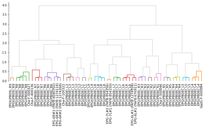
# Make cluster matching the color threshold in the dendrogram
clusters = fcluster(Z, t=.65, criterion='distance')
clusters

array([16, 14,  4,  5, 11,  4,  3, 12,  2, 19, 13,  4,  8,  3, 19,  2,  5,
       13,  3, 11, 17, 14, 16,  6, 12, 15, 18, 11, 12, 15, 15, 18,  5, 10,
        9,  2, 19,  8,  1,  9, 19,  3,  1, 10,  2,  9,  7, 18,  9,  2, 17,
       13, 12,  4, 17,  5,  7,  6,  4, 12, 16,  4], dtype=int32)

# We have to downsample the neurons for visualization 
# because DeepNote enforces a limit on the size of plots
eb_pb_ds = eb_pb.downsample(10)

# Make a color per cluster 
palette = sns.color_palette('tab20', max(clusters))
cmap = dict(zip(range(1, max(clusters) + 1), palette))

colors = [cmap[i] for i in clusters]

navis.plot3d(eb_pb_ds, color=colors)

3.9 - neuprint

The neuprint data and database

The Janelia hemibrain (Scheffer et al., 2020), MANC (Takemura et al., 2024) and male-cns (Berg et al., 2025) datasets are accessible via neuprint at https://neuprint.janelia.org. The web interface lets you run a few pre-built queries and you can also run custom queries directly against the underlying neo4j graph data base using cypher queries.

To access neuprint programmatically, we will use neuprint-python (link). It requires a free API token, which you can get by logging into the website using a Google account.

Getting started with neuprint-python

First we have to initialize the connection. Substitute {your_token} with your neuprint token.

import neuprint as neu
client = neu.Client('https://neuprint.janelia.org', dataset='hemibrain:v1.1',
                    token={your_token})

Most functions in neuprint-python accept neu.NeuronCriteria which is effectively a filter for body IDs, types, etc:

help(neu.NeuronCriteria)

Help on class NeuronCriteria in module neuprint.neuroncriteria:

class NeuronCriteria(builtins.object)
 |  NeuronCriteria(matchvar='n', *, bodyId=None, instance=None, type=None, regex=False, cellBodyFiber=None, status=None, cropped=None, min_pre=0, min_post=0, rois=None, inputRois=None, outputRois=None, min_roi_inputs=1, min_roi_outputs=1, label=None, roi_req='all', client=None)
 |  
 |  Specifies which fields to filter by when searching for a Neuron (or Segment).
 |  This class does not send queries itself, but you use it to specify search
 |  criteria for various query functions.
 |  
 |  Note:
 |      For simple queries involving only particular bodyId(s) or type(s)/instance(s),
 |      you can usually just pass the ``bodyId`` or ``type`` to the query function,
 |      without constructing a full ``NeuronCriteria``.
 |  
 |      .. code-block:: python
 |  
 |          from neuprint import fetch_neurons, NeuronCriteria as NC
 |  
 |          # Equivalent
 |          neuron_df, conn_df = fetch_neurons(NC(bodyId=329566174))
 |          neuron_df, conn_df = fetch_neurons(329566174)
 |  
 |          # Equivalent
 |          # (Criteria is satisfied if either type or instance matches.)
 |          neuron_df, conn_df = fetch_neurons(NC(type="OA-VPM3", instance="OA-VPM3"))
 |          neuron_df, conn_df = fetch_neurons("OA-VPM3")
 |  
 |  Methods defined here:
 |  
 |  __eq__(self, value)
 |      Implement comparison between criteria.
 |      Note: 'matchvar' is not considered during the comparison.
 |  
 |  __init__(self, matchvar='n', *, bodyId=None, instance=None, type=None, regex=False, cellBodyFiber=None, status=None, cropped=None, min_pre=0, min_post=0, rois=None, inputRois=None, outputRois=None, min_roi_inputs=1, min_roi_outputs=1, label=None, roi_req='all', client=None)
 |      Except for ``matchvar``, all parameters must be passed as keyword arguments.
 |      
 |      .. note::
 |      
 |          **Options for specifying ROI criteria**
 |      
 |          The ``rois`` argument merely matches neurons that intersect the given ROIs at all
 |          (without distinguishing between inputs and outputs).
 |      
 |          The ``inputRois`` and ``outputRois`` arguments allow you to put requirements
 |          on whether or not neurons have inputs or outputs in the listed ROIs.
 |          It results a more expensive query, but its more powerful.
 |          It also enables you to require a minimum number of connections in the given
 |          ``inputRois`` or ``outputRois`` using the ``min_roi_inputs`` and ``min_roi_outputs``
 |          criteria.
 |      
 |          In either case, use use ``roi_req`` to specify whether a neuron must match just
 |          one (``any``) of the listed ROIs, or ``all`` of them.
 |      
 |      Args:
 |          matchvar (str):
 |              An arbitrary cypher variable name to use when this
 |              ``NeuronCriteria`` is used to construct cypher queries.
 |              To help catch errors (such as accidentally passing a ``type`` or
 |              ``instance`` name in the wrong argument position), we require that
 |              ``matchvar`` begin with a lowercase letter.
 |      
 |          bodyId (int or list of ints):
 |              List of bodyId values.
 |      
 |          instance (str or list of str):
 |              If ``regex=True``, then the instance will be matched as a regular expression.
 |              Otherwise, only exact matches are found. To search for neurons with no instance
 |              at all, use ``instance=[None]``. If both ``type`` and ``instance`` criteria are
 |              supplied, any neuron that matches EITHER criteria will match the overall criteria.
 |      
 |          type (str or list of str):
 |              If ``regex=True``, then the type will be matched as a regular expression.
 |              Otherwise, only exact matches are found. To search for neurons with no type
 |              at all, use ``type=[None]``. If both ``type`` and ``instance`` criteria are
 |              supplied, any neuron that matches EITHER criteria will match the overall criteria.
 |      
 |          regex (bool):
 |              If ``True``, the ``instance`` and ``type`` arguments will be interpreted as
 |              regular expressions, rather than exact match strings.
 |      
 |          cellBodyFiber (str or list of str):
 |              Matches for the neuron ``cellBodyFiber`` field.  To search for neurons
 |              with no CBF at all, use ``cellBodyFiber=[None]``.
 |      
 |          status (str or list of str):
 |              Matches for the neuron ``status`` field.  To search for neurons with no status
 |              at all, use ``status=[None]``.
 |      
 |          cropped (bool):
 |              If given, restrict results to neurons that are cropped or not.
 |      
 |          min_pre (int):
 |              Exclude neurons that don't have at least this many t-bars (outputs) overall,
 |              regardless of how many t-bars exist in any particular ROI.
 |      
 |          min_post (int):
 |              Exclude neurons that don't have at least this many PSDs (inputs) overall,
 |              regardless of how many PSDs exist in any particular ROI.
 |      
 |          rois (str or list of str):
 |              ROIs that merely intersect the neuron, without specifying whether
 |              they're intersected by input or output synapses.
 |              If not provided, will be auto-set from ``inputRois`` and ``outputRois``.
 |      
 |          inputRois (str or list of str):
 |              Only Neurons which have inputs in EVERY one of the given ROIs will be matched.
 |              ``regex`` does not apply to this parameter.
 |      
 |          outputRois (str or list of str):
 |              Only Neurons which have outputs in EVERY one of the given ROIs will be matched.
 |              ``regex`` does not apply to this parameter.
 |      
 |          min_roi_inputs (int):
 |              How many input (post) synapses a neuron must have in each ROI to satisfy the
 |              ``inputRois`` criteria.  Can only be used if you provided ``inputRois``.
 |      
 |          min_roi_outputs (int):
 |              How many output (pre) synapses a neuron must have in each ROI to satisfy the
 |              ``outputRois`` criteria.   Can only be used if you provided ``outputRois``.
 |      
 |          roi_req (Either ``'any'`` or ``'all'``):
 |              Whether a neuron must intersect all of the listed input/output ROIs, or any of the listed input/output ROIs.
 |              When using 'any', each neuron must still match at least one input AND at least one output ROI.
 |      
 |          label (Either ``'Neuron'`` or ``'Segment'``):
 |              Which node label to match with.
 |              (In neuprint, all ``Neuron`` nodes are also ``Segment`` nodes.)
 |              By default, ``'Neuron'`` is used, unless you provided a non-empty ``bodyId`` list.
 |              In that case, ``'Segment'`` is the default. (It's assumed you're really interested
 |              in the bodies you explicitly listed, whether or not they have the ``'Neuron'`` label.)
 |      
 |          client (:py:class:`neuprint.client.Client`):
 |              Used to validate ROI names.
 |              If not provided, the global default ``Client`` will be used.
 |  
 |  __repr__(self)
 |      Return repr(self).
 |  
 |  all_conditions(self, *vars, prefix=0, comments=True)
 |  
 |  basic_conditions(self, prefix=0, comments=True)
 |      Construct a WHERE clause based on the basic conditions
 |      in this criteria (i.e. everything except for the "directed ROI" conditions.)
 |  
 |  basic_exprs(self)
 |      Return the list of expressions that correspond
 |      to the members in this NeuronCriteria object.
 |      They're intended be combined (via 'AND') in
 |      the WHERE clause of a cypher query.
 |  
 |  bodyId_expr(self)
 |  
 |  cbf_expr(self)
 |  
 |  cropped_expr(self)
 |  
 |  directed_rois_condition(self, *vars, prefix=0, comments=True)
 |      Construct the ```WITH...WHERE``` statements that apply the "directed ROI"
 |      conditions specified by this criteria's ``inputRois`` and ``outputRois``
 |      members.
 |      
 |      These conditions are expensive to evaluate, so it's usually a good
 |      idea to position them LAST in your cypher query, once the result set
 |      has already been narrowed down by eariler filters.
 |  
 |  global_vars(self)
 |  
 |  global_with(self, *vars, prefix=0)
 |  
 |  instance_expr(self)
 |  
 |  post_expr(self)
 |  
 |  pre_expr(self)
 |  
 |  rois_expr(self)
 |  
 |  status_expr(self)
 |  
 |  type_expr(self)
 |  
 |  typeinst_expr(self)
 |      Unlike all other fields, type and instance OR'd together.
 |      Either match satisfies the criteria.
 |  
 |  ----------------------------------------------------------------------
 |  Class methods defined here:
 |  
 |  combined_conditions(neuron_conditions, vars=[], prefix=0, comments=True) from builtins.type
 |      Combine the conditions from multiple NeuronCriteria into a single string,
 |      putting the "cheap" conditions first and the "expensive" conditions last.
 |      (That is, basic conditions first and the directed ROI conditions last.)
 |  
 |  combined_global_with(neuron_conditions, vars=[], prefix=0) from builtins.type
 |  
 |  ----------------------------------------------------------------------
 |  Data descriptors defined here:
 |  
 |  __dict__
 |      dictionary for instance variables (if defined)
 |  
 |  __weakref__
 |      list of weak references to the object (if defined)
 |  
 |  ----------------------------------------------------------------------
 |  Data and other attributes defined here:
 |  
 |  MAX_LITERAL_LENGTH = 3
 |  
 |  __hash__ = None

Fetching neurons

Let’s say we want to find all antennnal lobe projection neurons (PNs). Their type nomenclature adheres to {glomerulus}_{lineage}PN (e.g. DA1_lPN = DA1 glomerulus lateral lineage PN) for uniglomerular PNs and a M_{lineage}PN{tract}{type} (e.g. M_vPNml50 = “multiglomerular ventral lineage PN mediolateral tract type 50) for multiglomerular PNs.

To get them all, we need to use regex patterns (see this cheatsheet):

# Define the filter criteria
nc = neu.NeuronCriteria(type='.*?_.*?PN.*?', regex=True)

# Get general info for these neurons 
pns, roi_info = neu.fetch_neurons(nc)

print(f'{pns.shape[0]} PNs found.')

pns.head()

337 PNs found.

# Check that the regex did not have any accidental by-catch
pns['type'].unique()

array(['M_vPNml53', 'M_lvPNm32', 'M_lvPNm36', 'M_vPNml70', 'M_vPNml89',
       'VP1l+_lvPN', 'M_vPNml69', 'DM1_lPN', 'DM4_vPN', 'M_vPNml79',
       'VP4+_vPN', 'DA4l_adPN', 'M_vPNml87', 'DM4_adPN', 'M_vPNml83',
       'VA5_lPN', 'DA4m_adPN', 'M_lvPNm24', 'M_vPNml85', 'VP1l+VP3_ilPN',
       'M_vPNml77', 'M_vPNml84', 'VC1_lPN', 'M_lvPNm39', 'M_vPNml50',
       'DM2_lPN', 'VC5_lvPN', 'M_vPNml88', 'M_vPNml58', 'VP4_vPN',
       'DP1m_vPN', 'DP1m_adPN', 'DM5_lPN', 'VC5_adPN', 'M_vPNml80',
       'M_lvPNm25', 'VC3m_lvPN', 'VP3+_vPN', 'VP1m+_lvPN', 'DA3_adPN',
       'V_l2PN', 'M_vPNml56', 'VC3l_adPN', 'VM7v_adPN', 'DL5_adPN',
       'VM4_adPN', 'VM2_adPN', 'M_lvPNm40', 'DC4_vPN', 'V_ilPN',
       'M_vPNml74', 'Z_lvPNm1', 'DA1_lPN', 'DP1l_adPN', 'VM4_lvPN',
       'M_vPNml71', 'DP1l_vPN', 'M_lvPNm41', 'M_spPN5t10', 'DA1_vPN',
       'VC4_adPN', 'DM3_adPN', 'M_lvPNm45', 'VL1_vPN', 'M_lvPNm44',
       'M_vPNml78', 'M_vPNml67', 'M_adPNm5', 'M_smPNm1', 'DM6_adPN',
       'DL2d_adPN', 'M_adPNm6', 'M_adPNm8', 'M_lvPNm43', 'Z_vPNml1',
       'M_vPNml59', 'DA2_lPN', 'M_lPNm11A', 'M_vPNml52', 'DL2d_vPN',
       'VL2p_vPN', 'VA1d_adPN', 'M_lPNm11B', 'M_lvPNm48', 'M_lPNm11C',
       'M_lvPNm42', 'VA1v_vPN', 'M_vPNml68', 'M_vPNml55', 'M_vPNml62',
       'VL2a_vPN', 'M_vPNml60', 'M_vPNml65', 'VM5d_adPN', 'M_l2PNm16',
       'M_vPNml61', 'M_vPNml57', 'M_vPNml64', 'M_lv2PN9t49',
       'VP2+VC5_l2PN', 'M_spPN4t9', 'M_vPNml66', 'M_vPNml75', 'M_vPNml63',
       'M_vPNml72', 'M_lvPNm38', 'D_adPN', 'M_vPNml76', 'M_vPNml54',
       'DM3_vPN', 'M_vPNml86', 'DL3_lPN', 'VA4_lPN', 'VP1d_il2PN',
       'DC1_adPN', 'M_l2PN3t18', 'M_lvPNm35', 'DL4_adPN', 'M_lvPNm28',
       'M_lvPNm27', 'M_ilPNm90', 'M_l2PNl20', 'M_lvPNm29', 'VA7l_adPN',
       'M_lPNm13', 'M_l2PNl21', 'DL1_adPN', 'M_imPNl92', 'M_vPNml73',
       'M_ilPN8t91', 'M_l2PNm14', 'VP1d+VP4_l2PN1', 'M_lvPNm26',
       'DL2v_adPN', 'VP3+VP1l_ivPN', 'M_lvPNm33', 'VA1v_adPN',
       'VP3+_l2PN', 'M_l2PN10t19', 'VP4+VL1_l2PN', 'M_l2PNl22',
       'M_l2PNm15', 'M_lPNm11D', 'MZ_lv2PN', 'DC2_adPN', 'M_lvPNm46',
       'VC2_lPN', 'VM1_lPN', 'VM3_adPN', 'VM7d_adPN', 'M_lvPNm47',
       'M_lPNm12', 'DC3_adPN', 'VP2+_adPN', 'VP1m+VP2_lvPN2',
       'VP1m+VP2_lvPN1', 'VA6_adPN', 'VA7m_lPN', 'M_adPNm7', 'M_adPNm4',
       'VA1d_vPN', 'VA3_adPN', 'VL1_ilPN', 'M_l2PNl23', 'M_lvPNm31',
       'VP1m+VP5_ilPN', 'VL2p_adPN', 'MZ_lvPN', 'VP2_adPN', 'VA2_adPN',
       'VM5v_adPN', 'VP5+VP2_l2PN', 'VP5+VP3_l2PN', 'VP5+_l2PN',
       'M_vPNml51', 'M_smPN6t2', 'M_lvPNm37', 'M_vPNml82', 'M_adPNm3',
       'VP1m_l2PN', 'DC4_adPN', 'VP5+Z_adPN', 'VL2a_adPN', 'VP2_l2PN',
       'M_lvPNm34', 'VP2+Z_lvPN', 'M_lvPNm30', 'M_l2PNm17', 'M_vPNml81',
       'VP1d+VP4_l2PN2'], dtype=object)

Fetching synaptic partners

Looks good! Now let’s find neurons downstream of those PNs:

ds = neu.fetch_simple_connections(upstream_criteria=neu.NeuronCriteria(bodyId=pns.bodyId.values))
ds.head()

Each row shows the set of connections between two single neurons. The “weight” is the total number of synapses from the presyanptic neuron to the postsynaptic neuron. Let’s group by cell type (summing weights for each pair of types) to simplify:

by_type = ds.groupby(['type_pre', 'type_post'], as_index=False).weight.sum()
by_type.sort_values('weight', ascending=False, inplace=True)
by_type.reset_index(drop=True, inplace=True)
by_type.head()

Unsurprisingly, the strongest connections are between PNs and Kenyon Cells (KCs), since there are thousands of KCs. Now let’s find out where these connections occur:

adj, roi_info2 = neu.fetch_adjacencies(sources=neu.NeuronCriteria(bodyId=pns.bodyId.values),
                                       targets=neu.NeuronCriteria(type='KC.*?', regex=True))
roi_info2.head()                                       

  0%|          | 0/2 [00:00<?, ?it/s]

# Group by region of interest (ROI)
by_roi = roi_info2.groupby('roi').weight.sum()
by_roi.head()

roi
CA(R)         180526
NotPrimary      2737
PLP(R)            11
SCL(R)           498
SLP(R)          2008
Name: weight, dtype: int64

As expected, most of these synapses are in the mushroom body calyx. Let’s also plot this as a graph:

ax = by_roi.plot.bar()
ax.set_xlabel('')
ax.set_ylabel('PN to KC synapses')

Text(0, 0.5, 'PN to KC synapses')

Querying paths

Let’s say we want to find a set of connections starting from a PN and going all the way to a descending neuron (presumably leading to motor neurons in the VNC).

# First fetch the DNs
dns, _ = neu.fetch_neurons(neu.NeuronCriteria(type='(.*DN[^1]{0,}.*|Giant Fiber)', regex=True))
dns.head()

Neuprint lets you query paths from a single source to a single target. For multi-source or -target queries, your best bet is to download the entire graph and run the queries locally using networkx or igraph.

# Find all paths from A PN to A DNs 
paths = neu.fetch_shortest_paths(upstream_bodyId=pns.bodyId.values[0],
                                 downstream_bodyId=dns.bodyId.values[0],
                                 min_weight=10)
paths                                 

So it looks like there are three separate 7-hop paths to go from M_vPNml53 to DN1a. Let’s plot a graph for this.

Plotting graphs

There are various ways of plotting static graphs. In theory Jupyter notebooks lend themselves to interactive graphs too but unfortunately DeepNote does not yet support the required libraries (e.g. ipywidgets). That being said: if you want to run this locally or on Google colab, check out ipycytoscape.

There are numerous options to do this but we will use networkx to plot a static graph:

import networkx as nx 
import numpy as np

# Initialize the graph
G = nx.DiGraph()

# Generate edges from the paths
edges = []
for p in paths.path.unique():
    this_path = paths.loc[(paths.path == p)]
    this_edges = list(zip(this_path.values[:-1], this_path.values[1:]))

    for i in range(this_path.shape[0] - 1):
        edges.append([this_path.bodyId.values[i], this_path.bodyId.values[i + 1], this_path.weight.values[i + 1]])

# Add the edges 
G.add_weighted_edges_from(edges)

# Add some names to the nodes 
nx.set_node_attributes(G, paths.set_index('bodyId')['type'].to_dict(), name='name')

```python


```python
import matplotlib.pyplot as plt 

# Draw using a simple force-directed layout
pos = nx.kamada_kawai_layout(G)

# We could draw everything in one step but this way we have more control over the plot
fig, ax = plt.subplots(figsize=(10, 10))

# Draw nodes
nx.draw_networkx_nodes(G, pos=pos, ax=ax)

# Draw edges
weights = np.array([e[2]['weight'] for e in G.edges(data=True)])
nx.draw_networkx_edges(G, pos=pos, width=(weights / 12).tolist())

# Add node labels 
nx.draw_networkx_labels(G, pos=pos, labels=dict(G.nodes('name')), font_size=14)

# Turn axes of
ax.set_axis_off()

In general, I recommend exporting your graph to e.g. graphml and importing it into e.g. cytoscape if you want to explorate an interactive network graph.

nx.write_gml(G, "my_graph.gml")

<networkx.classes.digraph.DiGraph at 0x7f4ddb5c4d50>

G

<networkx.classes.digraph.DiGraph at 0x7f4ddb5c4d50>

Last but not least: let’s visualize the neurons involved!

Fetching meshes & skeletons

You can fetch skeletons as SWCs directly via neuprint-python. For visualization however it’s easiest to load neuron morphologies via navis. For that navis wraps neuprint-python and adds some convenience functions (see also the tutorial):

# Import the wrapped neuprint-python 
# -> this exposes ALL base functions plus a couple navis-specific extras
import navis
import navis.interfaces.neuprint as neu 

navis.set_pbars(jupyter=False)

client = neu.Client('https://neuprint.janelia.org', dataset='hemibrain:v1.1')

# Fetch neurons in the first path
nl = neu.fetch_skeletons(paths.loc[(paths.path == 0), 'bodyId'])
nl