Which fly is this?
The animal behind the data on Virtual Fly Brain — the species, the strains, the individual flies that were imaged, and the century of genetics that makes any of it interpretable.
Every image, neuron and connection on Virtual Fly Brain came out of a real animal. This page is about which animal: the species, the genetic background, and — for the electron microscopy volumes — the specific individual fly that was dissected on a specific morning. It also covers how a hundred years of Drosophila genetics produced the reagents and reference frames that let data from different laboratories be compared at all.
The short answer
Drosophila melanogaster: the fruit fly Thomas Hunt Morgan’s group bred in the Fly Room at Columbia, and the animal almost every technique described below was built around.
The more precise answer is that the connectomic data on VFB came from one laboratory cross, repeated — and in two cases, from a single individual whose brain and optic lobe were reconstructed separately.
The same cross, every time
The flagship EM volumes were not taken from a wild population or from a lab’s general stock. Every one of them is the F1 of a cross between the wild-type Canton-S strain G1 and w1118. The Janelia volumes were reared on a 12-hour day/night cycle and dissected 1.5 hours after lights-on; the direction of the cross as written varies between papers.
| Volume in VFB | Stage and sex | Age | Genotype | Source |
|---|---|---|---|---|
| FAFB / FlyWire | Adult female | 7 days post-eclosion | [iso] w1118 × [iso] Canton-S G1 | Zheng et al. (2018) |
| Hemibrain | Adult female | 5 days post-eclosion | Canton-S G1 × w1118 | Scheffer et al. (2020) |
| MANC (male VNC) | Adult male | 5 days post-eclosion | Canton-S G1 × w1118 | Takemura et al. (2024) |
| Optic lobe | Adult male | 5 days post-eclosion | Canton-S G1 × w1118 | Nern et al. (2025) |
| male-CNS | Adult male | 5 days post-eclosion | Canton-S G1 × w1118 | Berg et al. (2025) |
| BANC | Adult female | 5–6 days post-eclosion | F1 of w1118 × Canton-S | Bates et al. (2026) |
| L1 larval CNS | First-instar female larva | 6 hours after hatching | Canton-S G1 [iso] × w1118 [iso] 5905 | Winding et al. (2023), volume from Ohyama et al. (2015) |
Two rows of that table are the same individual fly. Both the optic lobe study and the
male-CNS study name their specimen Z0720-07m, selected as the best of 44 preparations
screened by X-ray CT; the male-CNS paper describes the optic lobe work as “an earlier
study of the same sample”. Counting neurons across those two datasets therefore
double-counts the same cells — the male-brain equivalent of the FlyWire/hemibrain problem
set out on the neuron counts page, except that here it is
literally one animal rather than two animals imaged in the same region.
Two further things follow from this table, and both matter when you read a result off VFB.
Each connectome is one animal. A connectome is not a population average; it is a census of the individual that was sectioned. Where two connectomes disagree about a neuron’s partners, the difference may be reconstruction, or it may be that flies differ. The neuron counts page works through what this does to any number you might want to quote, including the fact that FlyWire and the hemibrain partly re-reconstruct the same tissue.
Sex and stage are properties of the dataset, not of “the fly”. FAFB, the hemibrain and BANC are female; MANC, the optic lobe and male-CNS are male; the larval connectome is a six-hour-old first instar. A cell type present in one is not guaranteed to be present, or to have the same partners, in another — which is the point of the male-CNS study, which reports 7,205 isomorphic, 114 dimorphic, 262 male-specific and 69 female-specific types between the male and female brain connectomes (Berg et al., 2025). VFB keeps sex and stage on the dataset record for exactly this reason.
One of them was not a random fly. The BANC specimen was chosen by behaviour. The authors screened 5–6-day-old females and picked one that “turned right 70% of the time over 582 choices when walking in an acrylic Y-maze”, putting it “at the 97th percentile for handedness in the population (n = 1,095)” (Bates et al., 2026). That was a deliberate and reasonable choice — a strong behavioural phenotype makes the connectome more interpretable — but it means the BANC animal is a documented outlier on at least one axis, not a draw from the middle of the distribution. Worth knowing before treating it as typical.
What that genotype actually is
Both halves of the cross have FlyBase records, and reading them turns the genotype into a short history of the field.
Canton-S, or Canton-Special (FBsn0000274), is one of the standard wild-type laboratory strains. FlyBase records that it was “selected by C. Bridges”, and that “C. Bridges found that salivary chromosomes were normal” — the same Bridges whose salivary gland maps are cited below, vetting the stock with the technique he had just built. It is still distributed, by Bloomington (64349) and Kyoto (105666). The report also notes that it “contains a recessive for multiple thoracic and scutellar bristles, which overlaps wild type in most flies but appears sporadically in strains partly derived from Canton-S” — a useful reminder that “wild type” names a stock, not an absence of variation.
w1118 (FBal0018186) is a loss-of-function allele of the very gene Morgan reported in 1910: FlyBase gives the mutagen as spontaneous and the lesion as a “partial deletion of the w locus”, citing Hazelrigg et al. (1984) — the same paper that worked out how transduced copies of white behave, which is what made it usable as a transformation marker. It is the standard white-eyed background for transgenics, and not by accident: P-element and φC31 constructs are typically marked with mini-white — the P{GawB} enhancer-trap construct that produced many early GAL4 lines carries w+mW.hs (FBtp0000352) — and a white+ marker can only be scored in a white-mutant animal. The first mutant Morgan ever described is still the thing that tells you a transgene went in.
You can see this in VFB itself: driver line records carry genotypes such as
w[1118];P{w[+mW.hs]=GawB}c135, with the mutant background and the mini-white marker
both written out, and each links to its FlyBase report.
Crossing two isogenic stocks gives an F1 that is genetically uniform between individuals, so the specimen is reproducible in a way a wild-caught fly would not be. Isogenic backgrounds are also what the Drosophila Genetic Reference Panel exploits at population scale.
Light microscopy data is more varied — expression patterns are collected in whatever background the driver line lives in — but the same principle applies: an image is of one animal, and the templates exist to make many such animals comparable.
Why a fly at all
The fly’s advantage is not that it is simple. It is that a century of work has already been done on it, and the results were kept.
1910–1935: the chromosome theory. Morgan reported a white-eyed male and showed the trait was sex-linked (Morgan, 1910). His student Alfred Sturtevant used recombination frequencies between six sex-linked factors to place them in linear order — the first genetic map (Sturtevant, 1913). Hermann Muller showed X-rays induce mutations, turning mutation into something a laboratory could produce on demand (Muller, 1927). Calvin Bridges’ salivary gland chromosome maps gave a physical coordinate system to put the genetic one against (Bridges, 1935).
1978–1980: genetics as a way of finding genes by function. Ed Lewis worked out the bithorax complex and its role in segment identity (Lewis, 1978). Christiane Nüsslein-Volhard and Eric Wieschaus ran a saturation screen for mutations affecting the segmental pattern of the embryo, and in doing so demonstrated that a developmental programme could be enumerated gene by gene (Nüsslein-Volhard and Wieschaus, 1980). Lewis, Nüsslein-Volhard and Wieschaus shared the 1995 Nobel Prize in Physiology or Medicine “for their discoveries concerning the genetic control of early embryonic development”.
2000: the genome. The roughly 120-megabase euchromatic portion of the genome was sequenced by a whole-genome shotgun strategy, and reported to encode about 13,600 genes (Adams et al., 2000). Rubin and Lewis, reviewing the nine decades behind it, note that genetic and physical mapping, whole-genome mutational screens, and functional alteration of the genome by gene transfer were all pioneered in metazoans using this fly (Rubin and Lewis, 2000).
What accumulated alongside those results is the part that matters for VFB: balancer chromosomes that hold a mutation stable over generations, isogenic wild-type stocks, public stock centres that will post you a fly, and a curated genetic literature in FlyBase (Öztürk-Çolak et al., 2024) — which is why the strains named above can be looked up a century later, and why a driver line in a 2012 paper is still orderable today. FlyBase release FB2026_02 is current at the time of writing. For the history of the classical toolkit, Kaufman (2017) is the readable account; Hales et al. (2015) is a primer on the modern system; Bellen et al. (2010) covers what fly neuroscience gave vertebrate neuroscience.
What making one of these datasets actually involves
The reason the fly scales is that the bench work is cheap in everything except patience. Flies are reared in vials on a standard medium — the BANC animals, for instance, were “raised on standard cornmeal–dextrose medium at room temperature (around 20 °C) in natural lighting conditions” (Bates et al., 2026) — anaesthetised on CO2 to be sorted under a dissecting scope, and scored by eye, which is why so many classical markers are visible ones such as eye colour, wing shape and bristle morphology.
A typical light microscopy dataset on VFB is the end of a chain of crosses. Virgin females of one genotype are collected — they must be picked before they mate — and crossed to males of another. Where a genotype cannot be made homozygous, balancer chromosomes hold it stable. A balancer carries “one or more inverted sequences relative to a normal chromosome to prevent the recovery of exchange events”, so the arrangement it is paired with is passed on intact; to be useful it should also carry “a recessive lethal mutation not related to the lesion being balanced”, which stops the balancer going homozygous, and “a dominant visible mutation so that it can be easily followed in crossing schemes” (Kaufman, 2017). That is what lets a lethal mutation, or a chromosome carrying a particular set of transgenes, sit in a stock indefinitely and still be identified by eye in the next generation.
The animal is then dissected — a CNS is taken out under saline in a few minutes — fixed, immunostained (typically an antibody against the tag on the reporter, plus a neuropil counterstain such as nc82), mounted, and imaged on a confocal microscope. The stack is registered to a template, and only then does it become something that can be compared with anyone else’s data.
The EM datasets follow the same start and then diverge sharply in cost: the same rearing and dissection, then months of sectioning and imaging and, historically, years of tracing. See EM reconstruction.
What makes any of this reusable is that the reagents are public. Driver lines, balancers and effector stocks are distributed by stock centres — Bloomington, the VDRC, Kyoto — and catalogued in FlyBase, so a line named in a paper can be ordered and re-used (Zheng et al., 2024). VFB links each transgene record back to FlyBase and to the stock, which is usually what a user actually wants: not the image, but the reagent that produced it.
The techniques the data rests on
VFB is an integrator: nearly everything in it was generated by someone else, using one of a small number of methods. Each has a page.
| To get this | You need this | Page |
|---|---|---|
| Any transgene expressed in chosen cells | A binary expression system — GAL4/UAS, LexA/LexAop, Q | Binary expression systems |
| A pattern narrow enough to be one cell type | Split drivers — two hemidrivers intersecting | Split driver expression |
| One neuron’s shape out of a whole pattern | Stochastic labelling — FLP-out, MARCM, MCFO | Stochastic labelling |
| Images from different animals in one space | Registration to a standard template | Registration, Templates |
| Comparison between two template spaces | Bridging transforms | Bridging registrations |
| Synapse-level morphology and wiring | Volume EM, segmentation and proofreading | EM reconstruction, EM data |
| A wiring diagram you can query | Connectivity derived from those reconstructions | Connectivity |
| Which cells express which genes | Single-cell and single-nucleus RNA sequencing | scRNAseq data |
| “Is this the same neuron as that one?” | Morphological similarity scoring | NBLAST |
| A name that means the same thing across studies | An anatomy ontology | Cell types |
The reagent lineage, in one paragraph each
Getting DNA into the germline. Rubin and Spradling showed that P-element vectors could carry DNA into the Drosophila germline (Rubin and Spradling, 1982). Insertion site was uncontrolled, which mattered: where a construct lands affects how it is expressed. The φC31 integrase system fixed that by allowing insertion at a defined attP landing site, so two constructs can be compared without confounding position effects (Groth et al., 2004). Large insertion resources followed (Bellen et al., 2004; Venken et al., 2011), and CRISPR/Cas9 made targeted editing routine (Gratz et al., 2013).
Finding out where a gene is expressed. Enhancer traps put a reporter next to whatever regulatory element the transposon landed near, turning random insertion into a screen for expression patterns (O’Kane and Gehring, 1987).
Separating “where” from “what”. The decisive step was Brand and Perrimon’s adaptation of yeast GAL4. In their system the GAL4 gene “is inserted randomly into the Drosophila genome to drive GAL4 expression from one of a diverse array of genomic enhancers”, and a separate transgene carrying GAL4 binding sites in its promoter is activated wherever GAL4 is present — so one line supplies the pattern, another the payload, and the cross decides what happens where (Brand and Perrimon, 1993). Every driver line on VFB is downstream of this. See Binary expression systems.
Seeing anything at all. GFP made a live, genetically encoded reporter possible (Chalfie et al., 1994), which is what turns a driver line into an image.
Industrial-scale driver collections. Janelia built thousands of GAL4 lines from defined genomic fragments at a fixed landing site and imaged the CNS of each (Pfeiffer et al., 2008; Jenett et al., 2012 — 7,000 lines, image data published for 6,650). The Vienna Tiles collection characterised 7,705 enhancer candidates (Kvon et al., 2014). These two collections are the backbone of the light microscopy on VFB.
Making a pattern specific enough to be useful. Even a good GAL4 line usually labels more than one cell type. Splitting a transcription factor into an activation domain and a DNA-binding domain, each under a different enhancer, restricts expression to the intersection (Luan et al., 2006; Pfeiffer et al., 2010; Dionne et al., 2018). The scale of the effort this takes is worth stating: the Janelia resource reports 3,060 cell-type-specific split-GAL4 lines for the adult CNS and 1,373 characterised in third-instar larvae, drawn from the examination of over 77,000 split combinations between 2013 and 2023 (Meissner et al., 2025). Specificity is expensive. See Split driver expression.
Getting down to one neuron. Site-specific recombination (Golic and Lindquist, 1989) underpins MARCM (Lee and Luo, 1999) and MultiColor FlpOut (Nern et al., 2015). These produce the single-neuron light microscopy images that can be compared against EM reconstructions. See Stochastic labelling.
Putting everything in one coordinate frame. Nonrigid registration of confocal stacks onto a common template (Rohlfing and Maurer, 2003; Jefferis et al., 2007) is what makes cross-study comparison possible at all. The current standard, JRC2018, was built by groupwise registration — the unisex brain template from 62 individuals, 124 images counting left–right flips (Bogovic et al., 2020).
No single template ever won, so comparing across studies means bridging between them. The
transforms form a graph, maintained in the community navis-flybrains and nat.flybrains
packages so that everyone gets the same answer, and a conversion between two spaces is a
computed route through it — often several transforms deep:
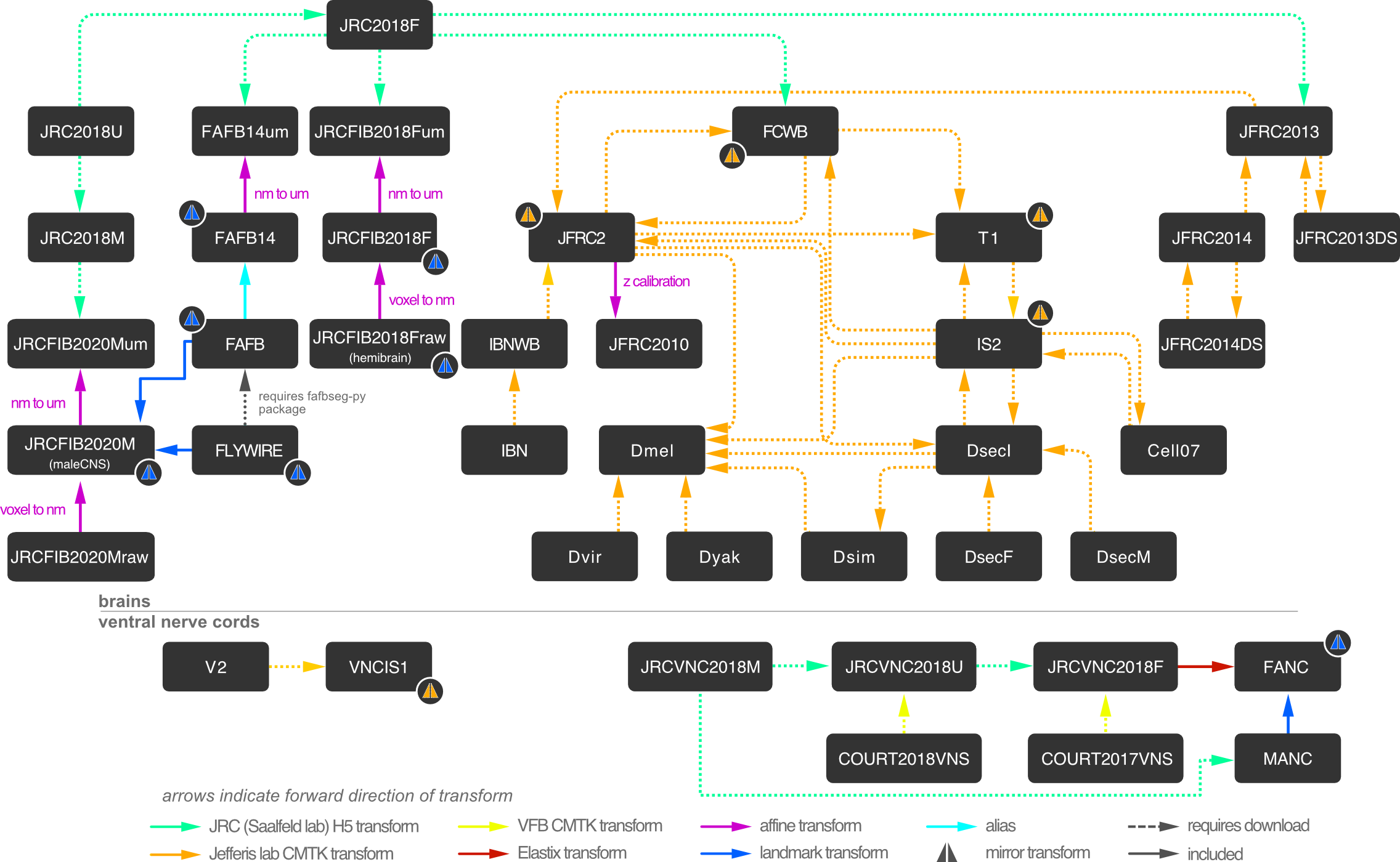
See Registration, Bridging registrations and Templates.
Wiring diagrams. Volume EM at synaptic resolution, then reconstruction: serial-section TEM for FAFB and the larval CNS (Bock et al., 2011; Zheng et al., 2018), FIB-SEM for the hemibrain, MANC and the optic lobe (Xu et al., 2017; Hayworth et al., 2015). Reconstruction moved from manual tracing in CATMAID (Saalfeld et al., 2009; Schneider-Mizell et al., 2016) to automated segmentation with human proofreading (Januszewski et al., 2018; Dorkenwald et al., 2022). See EM reconstruction.
Names. None of the above is comparable across studies without agreed terms. VFB is
built around the Drosophila Anatomy Ontology
(Costa et al., 2013), a manually curated,
queryable classification expressed in OWL. The schema behind it is a small, deliberate set
of relations — part_of and has_part, overlaps derived from them, and then the ones
that carry the neurobiology: has_soma_location, fasciculates_with,
has_synaptic_terminal_in with its pre- and post-synaptic forms, synapsed_to,
upstream_in_neural_path_with, innervates, develops_from
(Osumi-Sutherland et al., 2012). Properties
are asserted at the leaves and the hierarchy is left to a reasoner, because the alternative
does not scale: “a conventional relational database approach provides no means to automate
classification. Without this, maintaining the multiple inheritance classification schemes
biologists typically use quickly becomes impractical.” Built
from over 1,000 curated papers, the DAO represents some 13,000 neuroanatomical structures
and cell types, including over 9,800 terms for neuron types — of which more than 3,800 are
predicted from connectomics data
(Court et al., 2023). The region names came
in from outside: VFB “adapted and updated the Drosophila anatomy ontology to incorporate
the BrainName standard terminology”
(Milyaev et al., 2012), the community
standard later published as the systematic nomenclature for the insect brain
(Ito et al., 2014); the ventral nerve cord
got the same treatment
(Court et al., 2020). See
Cell types.
The ontology has its own inclusion rule, and it is the reason a VFB term can be treated as
evidence rather than opinion: the DAO includes a named class “only … where there is good
scientific evidence for the presence in wild-type animals of structures with the properties
described”, with links to the literature that supports it, and classes added in error have
been obsoleted. Terminology varies between groups and over time, so terms carry multiple
synonyms wherever possible, “linked to papers where they originate or that provide
examples of their usage”, with disambiguation comments where usage conflicts — which is
why searching VFB for an old or lab-specific name still finds the right structure. Much of
the classification is not hand-asserted but inferred: relations such as part_of and
capable_of, combined with Gene Ontology process terms and property chains, let a
reasoner derive the hierarchy and let disjointness axioms catch contradictions
(Costa et al., 2013).
How an image becomes a queryable fact. The bridge between the pictures and the
ontology is that images are modelled as OWL individuals. The painted neuropil domains on
a template are individuals of the relevant class, tied to it by a has_exemplar axiom, so
a term page can find its own illustration with a query. Every other image — single neuron,
clone, expression pattern — is registered onto that same template, and image analysis of
which regions it overlaps is written back as a type assertion on the individual. That is
what makes “show me neurons with a synaptic terminal in the antennal lobe” answerable at
all: the answer is inferred, not looked up. Reasoning propagates over partonomy through
property chains on overlaps and its subproperties — fasciculates_with,
has_synaptic_terminal_in — so a query at one level of the part hierarchy also returns
what was asserted further down it
(Osumi-Sutherland et al., 2014).
There is a deliberate design trade-off here. To keep reasoning fast enough to run live, the ontology is confined almost entirely to the EL profile of OWL, which is what allows the ELK reasoner to classify it in well under a second. The cost is expressiveness: EL has no negation, which is why the ontology-level compound queries were built to combine their legs with and. The 2014 paper makes the case that queries such as “neurons that synapse in the mushroom body but not in the lateral horn” would be genuinely useful for choosing specific reagents, and sets out closure-axiom and disjointness patterns that could support them (Osumi-Sutherland et al., 2014). What the current interface offers is documented under search and query.
VFB itself began as an interface onto that idea. The original paper describes two aims — “a hub for neuro-anatomical data integration” and “an easily accessible and usable tool to disseminate community agreed anatomical standards” — built over the BrainName reference stack for the adult brain, with queries answered by an OWL2 reasoner rather than by lookup, so that asking for neurons with presynaptic terminals in one region and postsynaptic terminals in another was a question the ontology could answer (Milyaev et al., 2012). The templates, datasets and connectomes described on this page were added to that frame.
What to keep in mind when you use VFB
- A cell type is an abstraction over individuals. When VFB says two images are the same cell type, that is a curatorial or computational judgement about neurons in different animals, not an observation of the same cell twice.
- Sex, stage and background travel with the dataset. Check them before comparing. The adult connectomes are not all the same sex, and the larval one is a different animal entirely.
- Registration is lossy. A neuron in template space is an estimate of where it was in its own brain. Bridging between templates compounds this.
- Predictions are labelled as such. Neurotransmitter assignments in the connectomes are predictions from EM image features, not measurements (Eckstein et al., 2024); see confidence values.
Sources
History and background
- Morgan TH (1910) Sex limited inheritance in Drosophila. Science 32(812):120–122. doi:10.1126/science.32.812.120
- Sturtevant AH (1913) The linear arrangement of six sex-linked factors in Drosophila, as shown by their mode of association. J Exp Zool 14:43–59. doi:10.1002/jez.1400140104
- Muller HJ (1927) Artificial transmutation of the gene. Science 66(1699):84–87. doi:10.1126/science.66.1699.84
- Bridges CB (1935) Salivary chromosome maps. J Hered 26:60–64. doi:10.1093/oxfordjournals.jhered.a104022
- Lewis EB (1978) A gene complex controlling segmentation in Drosophila. Nature 276:565–570. doi:10.1038/276565a0
- Nüsslein-Volhard C, Wieschaus E (1980) Mutations affecting segment number and polarity in Drosophila. Nature 287:795–801. doi:10.1038/287795a0
- Adams MD et al. (2000) The genome sequence of Drosophila melanogaster. Science 287(5461):2185–2195. doi:10.1126/science.287.5461.2185
- Rubin GM, Lewis EB (2000) A brief history of Drosophila’s contributions to genome research. Science 287(5461):2216–2218. doi:10.1126/science.287.5461.2216
- Bellen HJ, Tong C, Tsuda H (2010) 100 years of Drosophila research and its impact on vertebrate neuroscience. Nat Rev Neurosci 11:514–522. doi:10.1038/nrn2839
- Hales KG et al. (2015) Genetics on the fly: a primer on the Drosophila model system. Genetics 201:815–842. doi:10.1534/genetics.115.183392
- Kaufman TC (2017) A short history and description of Drosophila melanogaster classical genetics. Genetics 206:665–689. doi:10.1534/genetics.117.199950
- Mackay TFC et al. (2012) The Drosophila melanogaster Genetic Reference Panel. Nature 482:173–178. doi:10.1038/nature10811
- Öztürk-Çolak A et al. (2024) FlyBase: updates to the Drosophila genes and genomes database. Genetics 227:iyad211. doi:10.1093/genetics/iyad211
- Zheng S et al. (2024) An introductory guide to using Bloomington Drosophila Stock Center and FlyBase for aging research. Cells 13:1192. doi:10.3390/cells13141192
FlyBase records for the strains above (release FB2026_02)
- Canton-S — strain report FBsn0000274
- w1118 — allele report FBal0018186
- P{GawB}, carrying the mini-white marker w+mW.hs — construct report FBtp0000352
Specimens behind the EM volumes
- Zheng Z et al. (2018) A complete electron microscopy volume of the brain of adult Drosophila melanogaster. Cell 174(3):730–743. doi:10.1016/j.cell.2018.06.019
- Scheffer LK et al. (2020) A connectome and analysis of the adult Drosophila central brain. eLife 9:e57443. doi:10.7554/eLife.57443
- Takemura S et al. (2024) A connectome of the male Drosophila ventral nerve cord. eLife 13:RP97769. doi:10.7554/eLife.97769.1 — reviewed preprint
- Nern A et al. (2025) Connectome-driven neural inventory of a complete visual system. Nature 641:1225–1237. doi:10.1038/s41586-025-08746-0
- Berg S et al. (2025) Sexual dimorphism in the complete connectome of the Drosophila male central nervous system. bioRxiv 2025.10.09.680999. doi:10.1101/2025.10.09.680999 — preprint
- Bates AS et al. (2026) Distributed control circuits across a brain-and-cord connectome. Nature. doi:10.1038/s41586-026-10735-w
- Ohyama T et al. (2015) A multilevel multimodal circuit enhances action selection in Drosophila. Nature 520:633–639. doi:10.1038/nature14297
- Winding M et al. (2023) The connectome of an insect brain. Science 379(6636):eadd9330. doi:10.1126/science.add9330
- Dorkenwald S et al. (2024) Neuronal wiring diagram of an adult brain. Nature 634:124–138. doi:10.1038/s41586-024-07558-y
- Schlegel P et al. (2024) Whole-brain annotation and multi-connectome cell typing of Drosophila. Nature 634:139–152. doi:10.1038/s41586-024-07686-5
Techniques
- Rubin GM, Spradling AC (1982) Genetic transformation of Drosophila with transposable element vectors. Science 218:348–353. doi:10.1126/science.6289436
- Hazelrigg T, Levis R, Rubin GM (1984) Transformation of white locus DNA in Drosophila: dosage compensation, zeste interaction, and position effects. Cell 36:469–481. doi:10.1016/0092-8674(84)90240-X
- O’Kane CJ, Gehring WJ (1987) Detection in situ of genomic regulatory elements in Drosophila. PNAS 84:9123–9127. doi:10.1073/pnas.84.24.9123
- Golic KG, Lindquist S (1989) The FLP recombinase of yeast catalyzes site-specific recombination in the Drosophila genome. Cell 59:499–509. doi:10.1016/0092-8674(89)90033-0
- Brand AH, Perrimon N (1993) Targeted gene expression as a means of altering cell fates and generating dominant phenotypes. Development 118:401–415. doi:10.1242/dev.118.2.401
- Chalfie M et al. (1994) Green fluorescent protein as a marker for gene expression. Science 263:802–805. doi:10.1126/science.8303295
- Lee T, Luo L (1999) Mosaic analysis with a repressible cell marker for studies of gene function in neuronal morphogenesis. Neuron 22:451–461. doi:10.1016/S0896-6273(00)80701-1
- Rohlfing T, Maurer CR (2003) Nonrigid image registration in shared-memory multiprocessor environments. IEEE Trans Inf Technol Biomed 7:16–25. doi:10.1109/TITB.2003.808506
- Groth AC et al. (2004) Construction of transgenic Drosophila by using the site-specific integrase from phage φC31. Genetics 166:1775–1782. doi:10.1534/genetics.166.4.1775
- Bellen HJ et al. (2004) The BDGP gene disruption project. Genetics 167:761–781. doi:10.1534/genetics.104.026427
- Luan H et al. (2006) Refined spatial manipulation of neuronal function by combinatorial restriction of transgene expression. Neuron 52:425–436. doi:10.1016/j.neuron.2006.08.028
- Jefferis GSXE et al. (2007) Comprehensive maps of Drosophila higher olfactory centers. Cell 128:1187–1203. doi:10.1016/j.cell.2007.01.040
- Pfeiffer BD et al. (2008) Tools for neuroanatomy and neurogenetics in Drosophila. PNAS 105:9715–9720. doi:10.1073/pnas.0803697105
- Saalfeld S et al. (2009) CATMAID: collaborative annotation toolkit for massive amounts of image data. Bioinformatics 25:1984–1986. doi:10.1093/bioinformatics/btp266
- Pfeiffer BD et al. (2010) Refinement of tools for targeted gene expression in Drosophila. Genetics 186:735–755. doi:10.1534/genetics.110.119917
- Bock DD et al. (2011) Network anatomy and in vivo physiology of visual cortical neurons. Nature 471:177–182. doi:10.1038/nature09802
- Venken KJT et al. (2011) MiMIC: a highly versatile transposon insertion resource for engineering Drosophila melanogaster genes. Nat Methods 8:737–743. doi:10.1038/nmeth.1662
- Jenett A et al. (2012) A GAL4-driver line resource for Drosophila neurobiology. Cell Rep 2:991–1001. doi:10.1016/j.celrep.2012.09.011
- Osumi-Sutherland D et al. (2012) A strategy for building neuroanatomy ontologies. Bioinformatics 28:1262–1269. doi:10.1093/bioinformatics/bts113
- Gratz SJ et al. (2013) Genome engineering of Drosophila with the CRISPR RNA-guided Cas9 nuclease. Genetics 194:1029–1035. doi:10.1534/genetics.113.152710
- Ito K et al. (2014) A systematic nomenclature for the insect brain. Neuron 81:755–765. doi:10.1016/j.neuron.2013.12.017
- Kvon EZ et al. (2014) Genome-scale functional characterization of Drosophila developmental enhancers in vivo. Nature 512:91–95. doi:10.1038/nature13395
- Hayworth KJ et al. (2015) Ultrastructurally smooth thick partitioning and volume stitching for large-scale connectomics. Nat Methods 12:319–322. doi:10.1038/nmeth.3292
- Nern A, Pfeiffer BD, Rubin GM (2015) Optimized tools for multicolor stochastic labeling reveal diverse stereotyped cell arrangements in the fly visual system. PNAS 112:E2967–E2976. doi:10.1073/pnas.1506763112
- Costa M et al. (2016) NBLAST: rapid, sensitive comparison of neuronal structure and construction of neuron family databases. Neuron 91:293–311. doi:10.1016/j.neuron.2016.06.012
- Schneider-Mizell CM et al. (2016) Quantitative neuroanatomy for connectomics in Drosophila. eLife 5:e12059. doi:10.7554/eLife.12059
- Xu CS et al. (2017) Enhanced FIB-SEM systems for large-volume 3D imaging. eLife 6:e25916. doi:10.7554/eLife.25916
- Dionne H et al. (2018) Genetic reagents for making split-GAL4 lines in Drosophila. Genetics 209:31–35. doi:10.1534/genetics.118.300682
- Januszewski M et al. (2018) High-precision automated reconstruction of neurons with flood-filling networks. Nat Methods 15:605–610. doi:10.1038/s41592-018-0049-4
- Bogovic JA et al. (2020) An unbiased template of the Drosophila brain and ventral nerve cord. PLoS ONE 15(12):e0236495. doi:10.1371/journal.pone.0236495
- Court R et al. (2020) A systematic nomenclature for the Drosophila ventral nerve cord. Neuron 107:1071–1079. doi:10.1016/j.neuron.2020.08.005
- Dorkenwald S et al. (2022) FlyWire: online community for whole-brain connectomics. Nat Methods 19:119–128. doi:10.1038/s41592-021-01330-0
- Eckstein N et al. (2024) Neurotransmitter classification from electron microscopy images at synaptic sites in Drosophila melanogaster. Cell 187:2574–2594. doi:10.1016/j.cell.2024.03.016
- Meissner GW et al. (2025) A split-GAL4 driver line resource for Drosophila neuron types. eLife 13:RP98405. doi:10.7554/eLife.98405
Virtual Fly Brain
- Milyaev N et al. (2012) The Virtual Fly Brain browser and query interface. Bioinformatics 28:411–415. doi:10.1093/bioinformatics/btr677
- Costa M, Reeve S, Grumbling G, Osumi-Sutherland D (2013) The Drosophila anatomy ontology. J Biomed Semantics 4:32. doi:10.1186/2041-1480-4-32
- Osumi-Sutherland D, Costa M, Court R, O’Kane CJ (2014) Virtual Fly Brain — using OWL to support the mapping and genetic dissection of the Drosophila brain. Proceedings of OWLED 2014, CEUR Workshop Proceedings 1265:85–96. PDF
- Court R et al. (2023) Virtual Fly Brain — an interactive atlas of the Drosophila nervous system. Front Physiol 14:1076533. doi:10.3389/fphys.2023.1076533